Journal of The Institution of Engineers, Singapore Vol. 44 Issue 3 2004
NEURAL NETWORK TASK DECOMPOSITION BASED ON OUTPUT PARTITIONING Sheng-Uei Guan1*, Shanchun Li1 and Syn Kiat Tan1 ABSTRACT In this paper, we propose a new method for task decomposition based on output partitioning. The proposed method is able to find the appropriate architectures for largescale real-world problems automatically and efficiently. By using this method, a problem can be divided flexibly into several sub-problems as chosen, each of which is composed of the whole input vector and a fraction of the output vector. Each module (for each subproblem) is responsible for producing a fraction of the output vector of the original problem. Hence, the hidden structure for the original problem’s output units is decoupled. These modules can be grown and trained in sequence or in parallel. Incorporated with the constructive learning algorithm, our method does not require excessive computation and any prior knowledge concerning decomposition. The feasibility of output partitioning is analyzed and proved. Several benchmarks are implemented to test the validity of this method. Their results show that this method can reduce computation time, increase learning speed, and improve generalization accuracy for both classification and regression problems. BACKGROUND Multilayered feedforward neural networks are widely used for pattern classification, function approximation, prediction, optimization, and regression problems. When applied to larger-scale real-word problems (tasks), they still suffer some drawbacks, such as, the inefficiency in utilizing network resources as the task (and the network) gets larger, and the inability of the current learning schemes to cope with high-complexity tasks (G. Auda, M. Kamel and H. Raafat, 1996). Large networks tend to introduce high internal interference because of the strong coupling among their hidden-layer weights (R. A. Jacobs et. al., 1991). Internal interference exists during the training process: whenever updating the weights of hidden units, the influence (desired outputs) from several output units will cause the weights to compromise to non-optimal values due to the clash in their weight updating directions. A natural approach to overcome these drawbacks is to decompose the original task into several sub-tasks based on the “divide-and-conquer” technique. Up to now, various task decomposition methods have been proposed. These methods can be roughly classified into the following classes: 1) Functional Modularity. Different functional aspects in a 1
Department of Electrical and Computer Engineering, National University of Singapore, 10 Kent Ridge Crescent, Singapore 119260 *
[email protected]
78
Journal of The Institution of Engineers, Singapore Vol. 44 Issue 3 2004
task are modeled independently and the complete system functionality is obtained by the combination of these individual functional models (R. E. Jenkins and B. P. Yuhas, 1993). 2) Domain Decomposition. The original input data space is partitioned into several subspaces and each module (for each sub-problem) is learned to fit the local data on each sub-space, for example, the mixture of experts architecture (R. A. Jacobs et. al., 1991), and multi-sieving neural network (B. L. Lu et. al. 1994). 3) Class Decomposition. A problem is broken down into a set of sub-problems according to the inherent class relations among training data (B. L. Lu and M. Ito, 1999; R. Anand et. al., 1995). 4) State Decomposition. Different modules are learned to deal with different states in which the system can be at any time (V. Petridis and A. Kehagias, 1998). Class decomposition methods have been proposed for solving N-class problems. The method proposed in (R. Anand et. al., 1995) is to split an N-class problem into N twoclass sub-problems and each module is trained to learn a two-class sub-problem. Another method proposed in (B. L. Lu and M. Ito, 1999) divides an N-class problem into (N 2) two-class sub-problems. Each of the two-class sub-problems is learned independently while the existence of the training data belonging to the other N-2 classes is ignored. The final overall solution is obtained by integrating all of the trained modules into a min-max modular network. There are still some shortcomings to these proposed class decomposition methods. Firstly, these algorithms use predefined network architecture for each module to learn each subproblem. Secondly, these methods are only applied to classification problems. A more general approach applicable to not only classification problems but also other applications, such as regression, should be explored. Thirdly, they usually divide the problem into a set of two-class sub-problems. This will be an obvious limitation: when they are applied to a large-scale and complex N-class problem where N is large, a very large number of two-class sub-problems will have to be learned. In this paper, we propose a new and more general task decomposition method based on output partitioning to overcome these shortcomings mentioned above. In section 2, we will briefly describe our design goals. Then, the proposed task decomposition method will be depicted in section 3. The procedure for parallel growing and result merging will be illustrated in section 4. The experiments are implemented and analyzed in section 5. In section 6, we present an automatic output partition procedure for classification problems. Conclusions are presented in section 7. DESIGN GOALS In order to reduce excessive computation, increase learning speed, and improve generalization accuracy, the proposed method should meet the following design goals. Design goal 1: Instead of using predefined network structure, the neural network must automatically grow to an appropriate size without excessive computation. It is one of key issues in neural network design to find appropriate network architecture automatically for a given application and optimize the set of weights for the architecture. Constructive
79
Journal of The Institution of Engineers, Singapore Vol. 44 Issue 3 2004
learning algorithms (T. Y. Kwok and D. Y. Yeung, 1997) can tackle this problem. Constructive learning algorithms start with a small network and then grow additional hidden units and weights until a satisfactory solution is found. In this paper, we adopt the Constructive Backpropagation (CBP) algorithm (M. Lehtokangas, 1999). The reason why CBP is selected is that the implementation of CBP is simple and we only need to backpropagate the output error through one and only one hidden layer. This way the CBP algorithm is computationally as efficient as the popular Cascade Correlation (CC) algorithm (M. Lehtokangas, 1999; S. E. Fahlman and C. Lebiere, 1990). Design goal 2: Flexible decomposition method. We can decompose the original problem into a number of sub-problems as chosen (less than the number of output units). For a problem that has a high-dimensional output space, if we always split it into a set of single output sub-problems, the number of obtained modules will be very large. Instead, we can split it into a small number of modules each of which contains several output units. Another advantage of flexible decomposition is that sometimes we only want to know some portions of the results in the application. For example, for classification problems, there are some situations where we only want to find out whether the current pattern lies in some particular class or not. Design goal 3: A general decomposition method. The proposed method can be applied to not only classification problems but also regression problems with multiple output units. TASK DECOMPOSITION BASED ON OUTPUT PARTITIONING The decomposition of a large-scale and complex problem into a set of smaller and simpler sub-problems is the first step to implement modular neural network learning. Our approach is to split this complex problem with high-dimensional output space into a set of sub-problems with low-dimensional output spaces. Let ℑ be the training set for a problem with K-dimensional output space: ℑ = {(X p , T p )}p =1 P
(1)
where X p ∈ R N is the input vector of the pth training pattern, T p ∈ R K is the desired output vector for the pth training pattern, and P is the number of training patterns. Suppose we divide the original problem into s sub-problems, each with a Ki-dimensional (i = 1,2,…,s) output space:
{(
ℑi = X p , T pi
)}
P
(2)
p =1
where T pi ∈ R K i is the desired output vector of the pth training pattern for the ith subproblem.
80
Journal of The Institution of Engineers, Singapore Vol. 44 Issue 3 2004
Each sub-problem can be solved by growing and training a feedforward neural network (module). A collection of such modules is the overall solution of the original problem. In the following, we present why this method works. Many different cost functions (also called error measures) can be used for network training. The most commonly used one is the sum of squared errors and its variations: P
K
(3)
E = ∑∑ (o pk − t pk ) 2 p =1 k =1
where opk and tpk are the actual output value and desired output value of the kth output unit for the pth training pattern respectively. If we divide the output vector into s sections, each of which contains Ki output unit(s), then equation (3) can be transformed into: P
K
E = ∑∑ (o pk − t pk ) 2 p =1 k =1
K K1 + K 2 ⎤ ⎡ K1 2 2 2 ( o − t ) = ∑ ⎢∑ (o pk1 − t pk1 ) + ∑ (o pk2 − t pk2 ) + ⋅ ⋅ ⋅ + ∑ pk s pk s ⎥⎥ k s = K 1 + K 2 + ⋅⋅⋅ + K s −1 +1 p =1 ⎣ k1 =1 k 2 = K1 +1 ⎦ P
P
K1
P
= ∑ ∑ (o pk1 − t pk1 ) 2 + ∑ p =1 k1 =1
K1 + K 2
P
∑ (o pk 2 − t pk 2 )2 + ⋅ ⋅ ⋅ + ∑
p =1 k 2 = K 1 +1
= E1 + E 2 + ⋅ ⋅ ⋅ + E s
K
∑ (o
− t pk s ) 2
pk s p =1 k s = K 1 + K 2 + ⋅⋅⋅ + K s −1 +1
(4)
where K i ≥ 1, i = 1,2,..., s and K1 + K 2 + ⋅ ⋅ ⋅ + K s = K . Each E1, E2,…, Es is independent of each other and the only constraint among them is their sum E should be small enough (acceptable). We can make each module’s error small enough to gurantee the overall error small enough. We can divide the original problem into s sub-problems. Each sub-problem is composed of the whole input vector and a fraction of the output vector in the original problem. Obviously, the collection of s modules (for s sub-problems) is equivalent to the non-modular network. Furthermore, the hidden structures for the original problem’s output units are decoupled. This allows the hidden units in modular i to act more as feature detectors for the Ki output units than in a classic non-modular network. Consequently, weight modification in each module is guided by only one portion of the output units and learning is likely to be more efficient and the error to be smaller. Output partitioning to its extreme can be freed from internal interference caused from output clash - when each output is derived independently, the hidden units will not receive contradictory signals from several output units. Partitioning the output units into subsets reduce internal interference caused from output clash as each output subset is a
81
Journal of The Institution of Engineers, Singapore Vol. 44 Issue 3 2004
portion of the original output units, which means any internal interference within the subset will be less likely and will be a subset of the internal interference in the original network. PARALLEL GROWING AND RESULTS MERGING After problem decomposition, the original problem is divided into s sub-problems. Each sub-problem is solved by growing and training a module. So the original neural network for the original problem is replaced by the modular network, as shown in Figure 1. In the modular network architecture, each module can be grown and be trained in sequence or in parallel. When we apply the modules for new input data, each module is responsible for calculating a fraction of the output and their results are merged to generate the final output for the given data. The procedure for parallel growing and training modules to solve the original problem is shown in Figure 2. Firstly, divide the original problem into s sub-problems. Then construct s modules for the sub-problems. On the end, merge the results of sub-problems to form the solution for the original problem. For classification problems, we take the output unit among all sub-networks with the maximum value to be the class which the input sample belongs to. For regression problems, all outputs are used directly without any post-processing.
(a) Non-modular network
(b) Modular network based on output parallelism
Figure 1: Non-modular and modular network architecture
EXPERIMENTAL RESULTS AND ANALYSIS The Experiment Scheme Benchmark problems, namely, Building1, Vowel, and Letter Recognition, are used to evaluate the effectiveness of task decomposition based on output partitioning. Building1 problem is taken from the PROBEN1 benchmark collection (L. Prechelt, 1994) and it is a regression problem. The other two problems are taken from University of California at Irvine (UCI) repository of machine learning databases and are classification problems.
All networks used have a single hidden layer with hidden units added incrementally using the CBP algorithm (M. Lehtokangas, 1999) while the RPROP algorithm (M. Riedmiller
82
Journal of The Institution of Engineers, Singapore Vol. 44 Issue 3 2004
and H. Braun, 1993) is used to minimize the cost functions. In the set of experiments undertaken, Building1 and Vowel problem were conducted 20 runs and Letter Recognition problem was conducted 5 runs. 50%, 25%, and 25% of the problem’s total available patterns are used for training set, validation set, and testing set respectively. When a hidden unit needs to be added, 8 candidates are trained and the best one is selected. All the experiments are simulated on a Pentium III –650 PC. The sub-problems (modules) are solved sequentially and their CPU times expended are recorded respectively.
Figure 2: The parallel growing and results-merging procedure
RESULTS AND ANALYSIS Building1 Building1 problem has 14 inputs, 3 outputs, and 4208 patterns. It is divided into three sub-problems and each has only one output unit. Each sub-problem is solved by growing and training one module. From Table 1, we can see that test error reduction by modular network (0.483) vs. non-modular network (0.612) is 21.08%. The maximum training time consumed for the three modules is 79.80s, much less than that for the non-modular network (122.50s). It is noted that the amount of time expended for merging the modules to form the modular network and delivering the test patterns for obtaining the overall solution is little, about 0.35s (80.15s – 79.80s).
83
Journal of The Institution of Engineers, Singapore Vol. 44 Issue 3 2004
Vowel Vowel has 10 inputs, 11 outputs, and 990 patterns. The patterns were normalized and scaled so that each component lies within [0,1]. We divided the Vowel problem into eleven sub-problems and each has one output unit. From Table 1, we can see that the test error reduction is 20.78% and classification error reduction is as high as 29.89%. Meanwhile, training time for the modular network is 184.63s, less than one third of that for the non-modular network, 622.55s. Table 1: Performance comparison of modular network vs. non-modular network Problem
Max. of Epochs
Max. of Total of Total of Test C. T. Time Hidden Indp. Error Error (s) Units Param. (%) Non-modular 1891 122.50 6.80 167 0.612 Building1 (676) (42.99) (3.50) (63) (0.309) (3 outputs, Modular 1775 80.15 15.15 287 0.483 3 modules) (1195) (53.80) (9.27) (149) (0.092) Error Red. (%) 21.08 Non-modular 19264 622.55 26.65 707 4.557 34.737 Vowel (6277) (215.74) (9.05) (199) (0.800) (7.413) (11 outputs, Modular 23497 184.63 185.63 2349 3.610 24.355 11 modules) (7345) (57.51) (31.71) (380) (0.401) (4.382) Error Red. (%) 20.78 29.98 Non-modular 26292 64811.40 73.60 3607 1.214 21.672 Letter (5426) (10422.08) (18.72) (960) (0.036) (0.422) Recognition Modular 41531 11525.80 382.60 7711 0.896 15.784 (26 outputs, (14272) (3907.89) (29.59) (562) (0.015) (0.424) 13 modules) Error Red. (%) 26.19 27.17 Note: 1. “Max. of T. Time” stands for training time, the CPU time taken by growing and training each module or non-modular network. For the modular network, “Max. of T. Time” equals to the maximum training time of the modules plus the time expended for merging the modules to form the modular network and delivering the test patterns to obtain the overall solution. 2. “Total of Indp. Param.” stands for the total number of independent parameters (the number of weights and biases in the net) of all the modules. “C. Error” stands for classification error. “Error Red.” stands for the percentage of error reduction by modular network vs. non-modular network. 3. For the data, the first row is the average/sum and the second row is its standard deviation.
Letter Recognition Letter Recognition problem has 16 inputs, 26 outputs and 20000 patterns. Patterns were normalized and scaled to [0,1]. We divide Letter Recognition problem into thirteen subproblems with two output units each. From Table 1, the test error reduction is 26.19% and classification error reduction is as high as 27.17%. Training time for the modular network is 11525.80s compared to 64811.40s for the non-modular network.
From the experiments, we can see that their classification error and test error are reduced dramatically based on output partitioning. As to network complexity, it is unfair to compare the total number of independent parameters of the modular network with that of
84
Journal of The Institution of Engineers, Singapore Vol. 44 Issue 3 2004
the non-modular network. As we have expected, the former would usually be larger than the latter. However, each module has a distinctly different number of independent parameters, which explains why we should adopt a constructive learning algorithm instead of a predefined network architecture. OUTPUT PARTITIONING WITH FISHER’S LINEAR DISCRIMINANT (FLD) For Building and Vowel problems, we allocated a single sub-network for each output unit. Doing this is only possible for problems with few output units. To explore further the output partitioning concept, we present some suggestions on dividing a multi-class classification problem. Our heuristics starts by using a configuration of allocating two classes into one sub-network, then iteratively removing a sub-network by re-allocating its classes to other sub-networks based on a measure of classification difficulty. Automatic Output Partitioning The motivation to use several smaller sub-networks is to reduce the high internal interference inherent in large networks (R. A. Jacobs et. al., 1991) which has to classify all k classes in the problem. By dividing the problem into several sub-problems with distinct classes, we can reduce the internal interferences among classes, which cause classification errors. The main tenet of support vector machines (Bernhard S. and Alexander J. Smola, 2002) is that the class data near the decision boundary provides the most discriminating power to separate the classes. We would then try to locate k/2 pairs of classes such that they are the closest to each other and allocate a sub-network to each pair.
The following simple “greedy” approach is used: A suitable measure J(w) (we used Fisher’s criterion function in this paper) is calculated for all possible k(k-1) pairs of classes, where the value of J(w) decreases with the increasing difficulty of separating the two classes. These J(w) scores are first ranked in ascending order. Two classes that have the lowest J(w) score (i.e. the most difficult disjoint pair) are then chosen and assigned into a sub-network. All J(w) scores associated with the assigned pair are then removed from the list. Repeat until all classes have been assigned. For an odd number of classes, the final sub-network will classify three classes. This is not a problem as these final classes have the highest J(w) scores, and is the easiest set to classify. Fisher’s Linear Discriminant Fisher’s Linear Discriminant (FLD) (Duda R. O. and P.E. Hart, 1973) estimates the difficulty of separating two classes. FLD projects a d-dimensional feature space into a k-1 dimensional feature space, where d is the number of features and k is the number of classes. Working with pairs of classes, the projected feature space will be onedimensional (projected on one line).
Let a set of p training patterns be X = [x1,…xp]t, where each xi ∈ R n , i = [1, p] . These patterns belong to two classes. Let mj be the d-dimensional sample means as given by 85
Journal of The Institution of Engineers, Singapore Vol. 44 Issue 3 2004
mj =
1 nj
∑ x , where Xj represents the set of samples belonging to class
x∈ X j
j ∈1, 2 while nj
denote the total number of samples in class j. The sample means in the projected space is 1 j= 1 then given by m y = ∑ wt x =wt m j , where wt is the projection vector to map ∑ j n j y∈Y j n j x∈X j x to y. Defining the scatter for samples of class j as s j =
∑ (x − m )
x∈ X j
j
2
, the within-class scatter,
which measures how close the patterns in the same class are distributed, can be calculated 2
as
SW = ∑ s j
.
The
related
between-class
scatter
can
be
calculated
as
j =1
2
1 ∑ x is the mean of all patterns in the feature n x∈X j =1 space. We then calculate Fisher’s criterion function: S B = ∑ n j (m j − m)(m j − m)t , where m =
J ( w) =
wt S B w wt SW w
(5)
for which the optimal projection can be obtained by solving the eigenvector problem (SB - λjSW)wj = 0, where λj and wj are the non-zero eigenvalue/eigenvector pairs. The value of J(w) decreases with the increasing difficulty of separating the two classes. To reduce the k/2 number of sub-networks, we can iteratively remove the sub-network containing the classes with the highest J(w)values (i.e. easiest to classify). Each of these removed classes is then reassigned to other sub-networks containing the class having the next highest J(w)score. Experimental Results We examine the above automatic partitioning procedure on the Letter Recognition and Segmentation datasets. All configurations were repeated with 20 different sets of initial weights and results reported are the averages (standard deviations provided as well).
The Segmentation problem has 18 inputs, 7 outputs, and 2310 patterns. The patterns have been normalized and scaled so that each component lies within [0,1]. We first divide Segmentation into three sub-networks with 2, 2, 3 classes respectively. Next we apply the reduction procedure to obtain two sub-networks with 3, 4 classes respectively. We also showed two other configurations having three sub-networks – “furthest apart” and “random”. The partitioning for “furthest apart” is done similarly to the FLD method above, but here we choose pairs which are spaced furthest apart from each other. Using the “random” method to partition seven classes into three sub-networks with at least two classes each, there are 27C. 25C possible configurations; we only show one here for comparison.
86
Journal of The Institution of Engineers, Singapore Vol. 44 Issue 3 2004
From Table 2, we can see that the test error consistently reduced with more sub-networks used. Collectively, more hidden units are used with more sub-networks. The “furthest apart” method yield results worse than the conventional single network method. When the sub-network reduction procedure was applied, we see that the adding of new classes to a sub-network only increases its number of weights slightly. However, the test error obtained was consistently reduced as the number of sub-networks used increased. This is due to the decreased internal interference caused by fewer classes sharing the same set of input-to-hidden layer weights. We first divide the Letter Recognition problem into twelve sub-problems with the first 11th sub-networks each having two classes while the last sub-network has four (the final four classes have sufficiently large J(w)). Next, we apply the iterative reduction procedure and show the results with seven sub-networks. Results obtained were similar to the Segmentation problem. Table 2: Performance of automatic partitioning with FLD on classification problems Problem
Max. of Epochs
Max. of T. Time (s)
Total of Hidden Units
Total of Indp. Param.
Test Error
C. Error (%)
37425 (4984) 25089 (5932) 26785 (9287) 67087 (29357)
1811 (403) 1824 (49) 518 (150) 1334 (584)
28 (7) 38 (3) 52 (6) 80 (18)
815 (166) 941 (36) 1186 (105) 1771 (371)
1.288 (0.123) 1.257 (0.083) 1.167 (0.100) 1.306 (0.168)
5.858 (0.466) 5.503 (0.512) 5.095 (0.572) 5.650 (0.719)
29605 (12461)
570 (233)
49 (13)
1120 (246)
1.191 (0.133)
5.425 (0.595)
26292 64811 74 (5426) (10422) (19) Modular, 25386 7535 226 7 sub-networks (3458) (1861) (10) Modular, 33909 3586 349 12 sub-networks (6299) (651) (8) Refer to Table 1 for explanation of terms used in this table.
3607 (960) 4948 (268) 6764 (143)
1.214 (0.036) 1.041 (0.029) 0.924 (0.028)
21.672 (0.422) 18.316 (0.698) 16.808 (0.543)
Non-modular Segmentation (7 outputs)
Modular, 2 sub-networks Modular, 3 sub-networks Modular, 3 sub-networks (furthest apart) Modular, 3 sub-networks (random)
Non-modular
Letter Recognition (26 outputs)
Note:
CONCLUSIONS This paper presents an approach to task decomposition based on output partitioning. Feasibility of output partitioning is analyzed and proved by equation (4). A problem can be divided into several sub-problems, each of which is composed of the whole input
87
Journal of The Institution of Engineers, Singapore Vol. 44 Issue 3 2004
vector and a fraction of the output vector. Each module (for each sub-problem) thereby is responsible for producing a fraction of the output vector of the original problem. Such modules can be grown and trained in sequential or in parallel. Using task decomposition based on output partitioning, internal interference of a complex problem is greatly reduced. This is because the hidden structure for the original problem’s output units is decoupled and efficient and effective learning is consequently achieved. To facilitate automatic output partitioning, we presented an FLD-based approach to divide a problem into sub-problems and showed the results improved with the number of sub-networks used. REFERENCES G. Auda, M. Kamel and H. Raafat, “Modular neural network architectures for classification,” in IEEE International Conference on Neural Networks, Vol. 2, 1996, pp.1279-1284.
R. A. Jacobs and M. I. Jordan, M. I. Nowlan, and G. E. Hinton, “Adaptive mixtures of local experts,” Neural Computation, vol. 3, no. 1, pp.79-87, 1991. Federal Information Processing Standards Publication (1998). Analogue to Digital Conversion of Voice by 2400 bits/Second Mixed Excitation Linear Prediction (Draft). R. E. Jenkins and B. P. Yuhas, “A simplified neural network solution through problem decomposition: the case of the truck backer-upper,” IEEE Transactions on Neural Networks, vol. 4, no. 4, pp. 718 – 720, 1993. B. L. Lu, H. Kita, and Y. Nishikawa, “A multisieving neural-network architecture that decomposes learning tasks automatically,” in Proceedings of IEEE Conference on Neural Networks, Orlando, FL, 1994, pp. 1319-1324. B. L. Lu and M. Ito, “Task decomposition and module combination based on class relations: a modular neural network for pattern classification,” IEEE Transactions on Neural Networks, vol. 10, no. 5, pp. 1244 – 1256, 1999. R. Anand, K. Mehrotra, C. K. Mohan and S. Ranka, “Efficient classification for multiclass problems using modular neural networks,” IEEE Transactions on Neural Networks, vol. 6, no.1, pp. 117 – 124, 1995. V. Petridis and A. Kehagias, Predictive Modular Neural Network: Applications to Time Series, Kluwer Academic Publishers, Boston, 1998. T. Y. Kwok and D. Y. Yeung, “Objective functions for training new hidden units in constructive neural networks,” IEEE Transaction on Neural Networks, vol. 8, no. 5, pp.1131-1148, 1997.
88
Journal of The Institution of Engineers, Singapore Vol. 44 Issue 3 2004
M. Lehtokangas, “Modelling with constructive backpropagation,” Neural Networks, vol. 12, 1999, pp.707-716. S. E. Fahlman and C. Lebiere, “The cascade-correlation learning architecture,” in Advances in Neural Information Processing systems II, D. S. Touretzky, G. Hinton, and T. Sejnowski, Eds. San Mateo, CA: Morgan Kaufmann Publishers, 1990, pp.524532. L. Prechelt, “PROBEN1: A set of neural network benchmark problems and benchmarking rules,” Technical Report 21/94, Department of Informatics, University of Karlsruhe, Germany, 1994. M. Riedmiller and H. Braun, “A direct adaptive method for faster backpropagation learning: the RPROP algorithm,” in Proceedings of the IEEE International Conference on Neural Networks, 1993, pp.586-591. Duda R. O., and P.E. Hart, Pattern Classification and Scene Analysis, New York: Academic Express, 1973. Bernhard S. and Alexander J. Smola, Learning with Kernels, Cambridge, Massachusetts: The MIT Press, 2002.
89