Neural networks for relational learning: An experimental ... - CiteSeerX

Machine Learning manuscript No. (will be inserted by the editor)

Neural networks for relational learning: An experimental comparison Werner Uwents1 , Gabriele Monfardini2 Hendrik Blockeel1 , Marco Gori2 , Franco Scarselli2 1

Department of Computer Science, Katolieke Universiteit, Leuven, Belgium e-mail: {hendrik.blockeel,werner.uwents}@cs.kuleuven.ac.be

2

Dipartimento di Ingegneria dell’informazione Università di Siena, Siena, Italy e-mail: {marco,monfardini,franco}@dii.unisi.it

The date of receipt and acceptance will be inserted by the editor

Abstract In the last decade, connectionist models have been proposed that can process structured information directly. These methods, which are based on the use of graphs for the representation of the data and the relationships within the data, are particularly suitable for handling relational learning tasks. In this paper, two recently proposed architectures of this kind, i.e. Graph Neural Networks (GNNs) and Relational Neural Networks (RelNNs), are compared and discussed, along with their corresponding learning schemes. The goal is to evaluate the performance of these methods on benchmarks that are commonly used by the relational learning community. Moreover, we also aim at reporting differences in the behavior of the

2

Werner Uwents et al.

two models, in order to gain insights on possible extensions of the approaches. Since RelNNs have been developed with the specific task of learning aggregate functions in mind, some experiments are run considering that particular task. In addition, we carry out more general experiments on the mutagenesis and the biodegradability datasets, on which several other relational learners have been evaluated. The experimental results are promising and suggest that RelNNs and GNNs can be a viable approach for learning on relational data.

1 Introduction

Object localization [Bianchini et al., 2005], image classification [Francesconi et al., 1998], natural language processing [Krahmer et al., 2003], bioinformatics [Baldi and Pollastri, 2004], QSAR [Micheli et al., 2001], web page scoring, social network analysis [Newman, 2001] and relational learning are examples of application domains where the information of interest is encoded into a set of basic entities and relationships between them. In all these domains, the data is naturally represented by sequences, trees, and, more generally, directed or undirected graphs. In fact, nodes can denote concepts while edges can specify their relationships. A machine learning technique for graphical domains is formally described as a function ϕ, to be learned by examples, that computes a value ϕ(G, n), where G is a graph and n one of its

Neural networks for relational learning: An experimental comparison

3

nodes. Intuitively, ϕ(G, n) is a property of the concept n 1 that is predicted using all the known concepts and their relationships. For example, relational databases contain information that is naturally encoded as graphs: each tuple of a relation can be denoted by a node, while the relationships between different tuples are represented by edges (see Fig. 1). The nodes of the graph have labels (i.e., feature vectors of real numbers) which correspond to the fields of the tuples. Recently, the study of machine learning techniques for relational data has received an increasing interest from researchers. A common goal consists of predicting the value of a field, i.e. learning a function ϕ(G, n) from examples, that takes as input a database G, a tuple n and returns the value of a target field of n. In the case of Fig. 1, ϕ may be used to predict the customer ratings: ϕ exploits all the database information for the prediction; the training set consists of customers that have or have not payed their debts. In the last years, new connectionist models were proposed that are capable to take in input graphs and trees directly, embedding the relationships between nodes into the processing scheme [Hammer and Jain, 2004]. They extend support vector machines [Kondor and Lafferty, 2002, Gärtner, 2003], neural networks [Sperduti and Starita, 1997,Frasconi et al., 1998,Gori et al., 2005] and SOMs [Hagenbuchner et al., 2003] to structured data. The main idea underlying those methods is to

1

For sake of simplicity, in this paper, the formally correct sentences “the concept

represented by n” and “the relationship represented by (n, u)” are sometimes shortened to “the concept n” and “the relationship (n, u),” respectively.

4


name

address

sex

Mr A Rome Male Mr B Siena Male Mrs B London Female

: :

: :

rating

id

type

customer_id

id

Accounts_id

plain saving

2 ? 2

saving

: : : :

: :

Customers

: :

: :

: :

Accounts

[plain]

[out,10000]

[Siena,Male,?]

[saving]

[in,1000]

[saving]

[out,30000]

: :

Quantity 10,000 1,000 30,000

: :

: :

Transactions

[Rome,Male,2]

: :

In/out out in out

: :

Fig. 1 A relational database and its graphical representation. Tuples are represented by nodes and fields by node labels. The goal of a relational learner is to predict the unknown value of a tuple field (here represented by a question mark).

automatically obtain an internal flat representation of the symbolic and subsymbolic information collected in the graphs. In this paper, we focus on supervised learning and we discuss and experimentally evaluate two connectionist models that have been recently proposed, i.e. Relational Neural Networks (RelNNs) [Blockeel and Bruynooghe, 2003,Uwents and Blockeel, 2005] and Graph Neural Networks (GNNs) [Gori et al., 2005]. Those models are peculiar for two different reasons. RelNNs have been defined having relational learning in mind and their characteristics are specifically designed to obtain a good performance on tasks from such a field. On the other hand, the GNN model has been conceived to be general and to be able to process directly, i.e., without a


5

pre–processing, a very large class of graphs, including for instance, cyclic and undirected graphs. The paper experimentally evaluates the performance of those methods on benchmarks that are commonly adopted by the relational learning community. The results are promising and are comparable to the state of the art on benchmarks on QSAR problems, suggesting that RelNNs and GNNs can be a viable approach for learning on relational data. Moreover, we study and report differences in the behavior of the two models, in order to have insights on the possible extensions of the approaches. Actually, RelNNs and GNNs differ for the connectionist components they exploit, for the kind of graphs they can process and for the learning algorithm. The analysis of the experimental results aims to evaluate how each difference affects the performance and, more generally, the capabilities of the two models. The paper is organized as follows. In the next section, we review RelNNs, GNNs and some literature on connectionist models for graph processing. Section 3 describes the experimental comparison. Finally, the conclusions are drawn in Section 4.

2 Graph processing by neural networks

There exists an extensive literature on the application of neural networks to structured data domains. In this section, a quick overview of a number of approaches is given and GNNs and RelNNs are situated with regard to other methods. In order to reach such a goal, we introduce a general framework that is useful to formally describe the considered techniques.

6


In the following, a graph G is a pair (N ,E), where N is a set of nodes (or vertices), and E is a set of edges (or arcs) between nodes: E ⊆ {(u, v)|u, v ∈ N }. We assume that edges are directed, i.e. each edge (u, v) is ordered and it has a head v and a tail u. The children ch[n] of a node n are defined by ch[n] = {u| (n, u) ∈ E}. Finally, a graph is called acyclic if there is no path, i.e. a sequence of connected edges, that starts and ends in the same node2, otherwise it is cyclic. Connectionist models for graph processing assume that the data can be represented as directed graphs, standing for a set of concepts (the nodes) connected by relationships (the edges). The direction of each edge represents the dependence of a concept on another one, i.e. the edge (n, u) denotes the fact that concept n can be defined using concept u. Moreover, each node n has a feature vector of real values ln , called label, that describes some properties of the concept. In order to implement this idea, a real vector xn ∈ IRs , called state, is attached to each node n (see Fig. 2). The state should contain a description of the concept represented by the node, so the state of a node naturally depends on its label and on its children. Formally, xn is computed by a parametric function fwn , called state transition function, that combines the information attached to node n and to its children ch[n] xn = fwn (ln , xch[n] , lch[n] ),

n ∈ N,

(1)

where xch[n] and lch[n] are the states and the labels of the nodes in ch[n], respectively. The transition function f is implemented by a neural network and the parameters 2

not.

The considered paths can be of any length and be simple (without repeating nodes) or


7

x5 l5 l4

x4

x3 x1

l3 l1

x6

l6

x8

x2 l2

l8

x1 = fw ( l1 , x2 , x4 , x6 , l2 , l4 , l6 ) xch[1]

l ch[1]

Fig. 2 In a graph, nodes represent concepts and edges relationships. The state x1 is computed by the transition function that uses the label l1 of node 1, the states x2 , x4 , x6 and the labels l2 , l4 , l6 of the children of 1.

wn are the weights of this network. Although the transition function can adopt a different set of parameters for each node, as suggested by the notation wn , such a solution is not useful, since it would give rise to a model without generalization capability. In practice, only two solutions are used in the existing models: all the nodes share the same parameters, so that wn = w holds; a set of parameters is shared by a group of nodes and each node n has a type kn that defines the group it belongs to, i.e. wn = w kn . For example, in a dataset that represents a relational database, where nodes denote tuples, the type kn is naturally defined by the table the tuple n belongs to. It is worth noticing that if a node type is used, nodes having different type may even use different transition functions and feature vectors, i.e. kn may hold. ln ∈ IRdkn and fwn = fw kn

8


Moreover, for each node n an output vector on is also computed that depends on the state xn and the label ln of the node. The dependence is modeled by a parametric output function gwn

on = gwn (xn , ln ),

n ∈ N.

(2)

Together, equations (1) and (2) define a parametric model that computes an output on = ϕw (G, n) for each node n of the graph G, taking into account the labels and the relationships of all the nodes in G. The parameter set w includes all the w n used by the transition and the output functions3. Graph and relational neural networks are supervised learning models. In the supervised framework, the node output ϕw (G, n) predicts a property of the concept represented by n. Thus, a supervised learning set L can be defined as a set of triples L = {(Gi , ni,j , tni,j )| 1 ≤ i ≤ p, 1 ≤ j ≤ qi }, where each triple (Gi , ni,j , tni,j ) denotes a graph Gi , one of its nodes ni,j and the desired output tni,j . Moreover, p is the number of graphs in L and qi is the number of the supervised nodes in graph Gi , i.e. the nodes for which a desired output is given. The goal of the learning 3

Different versions of Eqs. (1) and (2) can be used, without affecting or even improving

the expressive power of the model. For instance, a more general model can process also graphs edge labels by including their codings into the inputs of fw , i.e., replacing Eq. (1) by xn = fw n (ln , xch[n] , led[n] , lch[n] ), where led[n] are the labels of the edges coming out from n. On the other hand, removing the node label from the input parameters of gw does not affect the expressive power, since such an information is already included in fw . In this paper, for sake of simplicity, we describe only the simplest general model that includes both GNNs and RelNNs.


9

procedure is to adapt the parameters w so that ϕw approximates the targets of supervised nodes. In practice, the learning problem is often implemented by the minimization of the quadratic error function

ew =

qi p X X

(tni,j − ϕw (Gi , ni,j ))2 .

(3)

i=1 j=1

As in common feedforward neural networks, several optimization algorithms can be used: almost all of them are based on a subprocedure that computes the error gradient w.r.t. the weights. When the gradient is available, the possible optimization methods include, for instance, gradient descent, scaled conjugate gradient, Levenberg– Marquardt and resilient backpropagation [Haykin, 1994]. RelNNs, GNNs and the other neural models for graph processing differ with regard to the implementation of the two functions fwn and gwn , and to the method adopted to compute the states xn and the gradient of the error function

∂ew ∂w .

Those

differences will be described in the following sections.

2.1 Learning algorithms

All the models we consider are based on a common idea. The graph processing defined by Eqs. (1) and (2) can also be described as the computation carried out on a large network, called encoding network, that has the same topology as the input graph. The encoding network is obtained by substituting all the nodes of G with “units” that compute the function fwn . The units are connected according to graph topology (Fig. 3), where the directions of the arcs are inverted. The “f -units” calculate the states locally at each node. The information is diffused

10

Werner Uwents et al. x5 , l 5

l5 l4

x1 , l 1

3

l6

x6 , l 6

x4 , l 4

fw l1

l5

5

4

l3

l3

fw

fw

l4

fw

x6 , l 6

1

x3 , l 3

fw

l6

6

l1

gw

x2 , l 2

3

l7

l2

l7

o3

fw

x2 , l 2

2

fw

7

l2

Fig. 3 A graph and the corresponding encoding network. The computation is carried out by “f -units” locally at each node and the information is diffused according to the graph connectivity. An output unit computes the output at node 3.

through the encoding network following the connections defined by the edges: while in the input graph edge directions express the dependencies between nodes, in the encoding network they define the direction of the information flow. For the nodes where the output is computed, the “f -unit” is also connected to another unit that implements the output function gwn . Actually, as clarified in the following, the encoding network can be used both to compute the states and to adapt the parameters. Since the encoding network connectivity depends on the input graph, in some approaches the input domain is limited in order to simplify the learning and the testing procedures. In fact, the main difference between RelNNs and GNNs is that the former model assumes that the input graph G is acyclic and has a root node4 . The root is the only supervised node and RelNNs produce just one output for each graph. Thus, RelNNs can be 4

A root node of the graph from which every other node is reachable.


11

adopted only on those tasks where the goal is to classify the concept represented by the whole graph, whereas GNNs make no assumption on the input domain and can produce a different output for each node, i.e. they can classify also the single concepts denoted by the nodes.

2.1.1 Relational neural networks

If a graph is acyclic, the corresponding encoding

network turns out to be a large feedforward neural network whose components are the neural network units implementing gwn and fwn (see Fig. 4). Thus, there is an order in which the units should be updated to propagate the signals from inputs to outputs. Going in the reverse direction, from outputs to inputs, makes it possible to backpropagate the error signal and compute the gradient. In other words, a common backpropagation procedure [McClelland et al., 1986] can be applied on the encoding network in order to obtain the states xn and the gradients

∂ew ∂wn .

More precisely, the states xn are evaluated by the networks fwn

following the natural order defined by the edges5 : first the states of the nodes without children are calculated, then the states of their parents, and so on until the state of the root is obtained. Finally, the output is produced by gwn . On the other hand, the gradient

∂ew ∂w

is calculated by backpropagating the error

from the root to the leaves. More precisely, the derivative of the error with respect to the node state

∂ew ∂xn

is computed first for the root, then for its children, and so on,

until the leaves are reached. For each unit, the value 5

∂ew ∂xn

allows to calculate the

Formally, an edge states that the concept represented by the parent node depends on the

concept denoted by the child. Thus, the set of edges define a partial order, called the natural order, that specify the dependencies between the concepts.

12

Werner Uwents et al. o1

gw

1

x1 , l 1 1

x2 , l 2

l2

l3

l1

fw

l1

fw

l4

x3 , l 3 l2

2

fw

x4 , l 4

l3

3

l6

l5

l4

4

x5 , l 5

l5

fw

fw

5

x6 , l 6

fw

6

l6

Fig. 4 An acyclic graph and the corresponding encoding network. The backpropagation learning algorithm can be used on the encoding network, which is a feedforward network.

gradient

∂ew ∂w n .

Finally, since the parameters are shared among nodes of the same

type, the corresponding gradients are accumulated. Such a learning algorithm, which is also used for recursive neural networks, is called backpropagation through structure [Sperduti and Starita, 1997, Frasconi et al., 1998].

Moreover, it is worth noting that, even if cyclic graphs cannot be taken in input directly by RelNNs, they can be transformed into trees by an appropriate pre– processing (see Fig. 5 and Algorithm 1). The procedure consists of unfolding the graphs into trees according to a breadth–first visit. The visit starts from the node n where the output is evaluated. At each step, a node u′ of the unfolding tree T along with a corresponding node u of the graph G are considered: T is extended by connecting u′ to a new set of children that are exact copies of the children of u. The procedure is repeated until T has reached a predefined depth. At the end, T is


13

made up of copies6 of the nodes of G such that each copy in T resembles a node in G both for its label and for its local connectivity. Even if in practical applications the unfolding tree often contains most of the original information, in theory the pre-processing may cause a loss of information, because it may happen that two different graphs and/nodes are unfolded to the same tree. On the other hand, a theoretical condition ensuring that the unfolding is lossless is described in [Bianchini et al., 2006], where it is proved that the generated tree contains the same information of the original graph, provided that all the edges are visited and the nodes have distinct labels. See [Blockeel and Bruynooghe, 2003] for a more detailed description of the unfolding procedure implicit in the RelNN processing scheme.

2.1.2 Graph neural networks

The input graph of a GNN, and as a consequence

the encoding network, can be cyclic. In this case, backpropagation through structure cannot be used to compute the states and to train the network. Thus, three issues have to be addressed in order to implement GNNs: (a) as the states xn are defined recursively, depending one on the other, it must be ensured that they are defined unambiguously; (b) a method must be designed to compute the states xn ; (c) an algorithm is required to compute the gradient

∂ew ∂w .

Those issues are addressed in

the following. 6

In general, for each node in G there may exist several copies in T . Even if the number of

nodes grows exponentially with respect to the tree depth, it is possible to merge the common sub–structures whose dimension is linear with respect to the tree depth, as explained in Sect. 2.1.3.

14

Werner Uwents et al. 1

1

2

5

3

4

4

5

1

1

2

3

5

4 2 4

1

1

3

2

5

5

5

4

:

3

5

2

4

4

:

:

(A)

5

2

5

3

4

4

5

:

:

3

5

(B)

(C)

Fig. 5 A graph (A), its unfolding tree (B) and the corresponding directed acyclic graph (C). The tree (B) is generated visiting the graph (A) with a breadth-first strategy. Graph (C) is generated by merging common sub–trees in (B).

Algorithm 1 The unfolding algorithm Require: a graph G and one of its nodes n Build a tree T having a copy n′ of n as root Create an empty queue Q Q.push(n′ ) repeat u′ = Q.pop() Let u be the copy of u′ in G Let S be a set containing copies of the children ch[u] of u Extend T by connecting u′ to its children S Q.push(S) until G has been visited and T has reached a desired depth return T ;


15

– Existence and uniqueness of the states xn . Let F w and Gw be the vectorial functions obtained by stacking all the instances of fw and gw , respectively. Then Eqs. (1) and (2) can be rewritten for the GNN model as x = F w (x, l) ,

o = Gw (x, l) ,

(4)

where l represents the vector containing all the labels of the input graph and x collects all the states. By the Banach fixed point theorem [Khamsi, 2001], if F w is a contraction mapping7, then Eq. (4) has a unique solution. Thus, issue (a) can be solved by designing fw such that the global function F w results to be a contraction mapping w.r.t. the state x. In practice, this goal can be achieved by adding a penalty term p(Fw ) to the error function ew =

qi p X X (tni,j − ϕw (Gi , ni,j ))2 + βp(Fw ) i=1 j=1

where p(Fw ) is a penalty term measuring the contractivity of Fw and β is a predefined parameter balancing the importance of the penalty term with respect to the error achieved on patterns8 . More details can be found in [Gori et al., 2005, Scarselli et al., 2009b]. 7

A function ρ : IRn → IRn is a contraction mapping w.r.t. a vector norm k ·

k, if there exists a real number µ, 0 ≤ µ < 1, such that for any x1 , x2 ∈ IRn , kρ(x1 ) − ρ(x2 )k ≤ µkx 1 − x2 k. 8

More precisely, the proposed approach cannot ensure that the transition function Fw

is a contraction mapping outside of the training set. In theory, a GNN may not be able to compute a unique state, if it is applied on a graph which is different from those already observed in training set. However, in practice, such a case would not have any particular consequence except for the wrong prediction produced for the current input graph. More importantly, such a behaviour has never been observed in the experiments. It is also worth

16


– Computation of the states xn . The Banach fixed point theorem also suggests a method to solve issue (b). In fact, the theorem states that if F w is a contraction mapping, then the dynamical system x(t+1) = F w (x(t)), where x(t) denotes the proposed t–th iterate of x, converges exponentially fast to the solution of Eq. (4). In other words, the states can be simply computed by an iterative application of their definition, i.e. by the following dynamical system9 . xn (t) = fw (ln , xch[n] (t − 1), lch[n] ),

n∈N.

(5)

Intuitively, each iteration corresponds to an activation of the f-units in the encoding network. The computation is stopped when the state change becomes small, i.e. kx(t) − x(t − 1)k ≤ ε for a vectorial norm k · k and a predefined small real number ε. – Computation of the gradient. In order to design a gradient descent learning algorithm, we can observe that the encoding network represents a system having a settling behavior. For this reason, the gradient can be computed using the Almeida–Pineda algorithm [Almeida, 1990,Pineda, 1987]. In fact, GNNs compute the gradient by a combination of the backpropagation through structure algorithm and the Almeida–Pineda algorithm which consists of two phases: a) The states xn (t) are iteratively updated, using Eq. (5), until they are close to the fixed point at step r; mentioning that there exists another version of the GNN model, called linear GNN [Scarselli et al., 2009b], which does not suffer from this limitation and was not used in this paper since, according to previous experiments, its performance is lower. 9

Since, by Banach theorem, the fixed point is unique, the stable point computed by the

dynamical system does not depend on the initial state.


b) The gradient

∂ew ∂w

17

is calculated by backpropagating the error signal through

the encoding network from step r back to previous steps, until the error signal is close to 0. Then, the weights are updated. Thus, while phase (a) moves the system to a stable point, phase (b) adapts the weights to change the outputs towards the desired target. The two phases are iterated until some stop criterion is fulfilled. It is worth to mention that even if the gradient could be computed also by applying the standard backpropagation through time algorithm [Werbos, 1990] to the encoding network, however the procedure adopted by GNNs is faster and uses less memory by exploiting Almeida–Pineda algorithm peculiarities. More details can be found in [Gori et al., 2005, Scarselli et al., 2009b].

2.1.3 Computational complexity issues

The time computational cost of learning

in RelNNs is mainly due to the forward and the backward phases of the backpropagation algorithm. The two phases have linear cost with respect to the dimension of the encoding network. When the input graph is acyclic, the encoding network has exactly the same shape of the graph, so that each step of the learning algorithm costs O(max(|N |, |E|)), i.e., the cost is linear with respect to the number of nodes and the number of edges in G. A similar analysis applies to the case when the input graph is cyclic, provided that we consider the unfolding tree of G instead of G itself. One may wonder whether the dimension of unfolding trees is a problem, since the number of nodes grows exponentially with respect to the tree depth. However, unfolding trees can be easily reduced by merging the common sub–structures (see Fig. 5). In fact, two

18


nodes can be fused provided that they have the same label and their children have been already fused. Such a merging procedure can be repeated from leaves to root until, in each level of the tree, there are at most as many nodes as in G. The result is an acyclic graph with less than O(d·|N |) nodes, where d is the maximum depth of trees, that contains the same information of the original tree and can be processed by a RelNN. On the other hand, the GNN learning algorithm requires O(r · max(|N |, |E|)) operations, where r is the number of iterations needed to compute the state by Eq. (5). Such a claim is explained observing that both each iteration of Eq. (5) and each step of backpropagation costs O(max(|N |, |E|)) (see [Scarselli et al., 2009b] for more details). Interestingly, r is usually small due to the fact that the convergence to the fixed point is exponential. Thus, learning has a similar cost in RelNNs and in GNNs. The difference is mainly due to the values d and r, which, are determined in two different ways: in RelNN, d is a predefined parameter of the pre–processing procedure; in GNNs, r is dynamically determined during learning.

2.2 Transition and output functions RelNNs and GNNs differ also for the implementation of the transition and the output functions.

2.2.1 Relational neural networks

Relational neural networks have the following

peculiarities: – The output function gwn is implemented by a feedforward neural network.


19

– The transition function fwn , which does not use the labels ln , is implemented by a recurrent neural network rwn that combines the states and the labels of the children of each node n, storing the result into an internal state z(i) ∈ IRs (see Fig. 6 (A)). Formally,

z(i) = rwn (xchi [n] , lchi [n] , z(i − 1))

(6)

where chi [n] is the i-th child of n and z(0) = z 0 is a default initial value. The recurrent network processes a child at every time step i, following some predefined order, which depends on the considered application. The final internal state is then used as the state of the node, i.e., xn = z(|ch[n]|). Notice that different kinds of recurrent neural networks have been proposed and can be used to implement rwn as, for instance, fully recurrent networks and locally recurrent networks [Back and Tsoi, 1994]. It is also worth mentioning that the order according to which the children are processed may affect the performance of RelNNs, particularly when such an order is arbitrary and it does not depend on domain knowledge. However, previous experiments have shown that the importance of the issue can be mitigated by shuffling the children during the learning [Uwents and Blockeel, 2005]. – Nodes are grouped per type. Different networks are used for different types of nodes. Each network can have a different number of inputs and parameters. The weights are only shared between networks of the same type.

2.2.2 Graph neural networks

Graph neural networks have the following characteristics:

20

Werner Uwents et al. x1 x1

fw

l1

x3 , l 3

x4 , l 4

1

x2 , l 2

rw

z0

z(1)

rw

1

1

x2 , l 2

x3 , l 3

z(2)

rw

1

x4 , l 4

(A) x1 x1

+ fw

l1

x3 , l 3

x4 , l 4

hw x2 , l 2

hw

hw l1

x2, l 2

x3, l 3

x4, l 4

(B)

Fig. 6 The implementation of the transition function in RelNNs (A) and GNNs (B).

– No distinction is made between the nodes in the graph. All the nodes share the same transition function and the same output function, i.e., fwn = fw , gwn = gw and the same parameters w n = w. – In GNNs, the transition function fw is implemented as a sum of contributions (see Fig. 6 (B)). Each contribution is related to a child and is produced by a feedforward neural network hw that takes in input the state and the label of the considered child and the label of the node10 X

|ch[n]|

xn = fw (ln , xch[n] , lch[n] ) =

hw (ln , xchi [n] , lchi [n] ).

(7)

i=1 10

Interestingly, both RelNNs and GNNs use specialized versions of fw . Actually, hw in

Eq. (7) and rw in Eq. (6) are preferred to the general fw in Eq. (1), because they allow to easily deal with application domains where the number of children for each node is highly varying.


21

Notice that, differently from the RelNN solution, xn does not depend on the order in which the children are processed. Obviously, this latter technique is advantageous or not according whether, in the considered application domain, important information can be encoded by an order relationship between the children11. Interestingly, GNNs are apparently limited by the fact that the global transition function F w has to be a contraction map and that Eq. (7) is used in place of Eq. (1). On the other hand, GNNs have been proved to be able to approximate in probability any function ϕ on graphs under mild conditions on the input domain and on the set of considered functions. For instance, the universal approximation holds provided that ϕ is continuous with respect to the graph labels and any node of each input graph can be distinguished from the other nodes either by mean of the label (the nodes have different labels) or by mean of the connectivity (the nodes belong to different paths). The result holds for non–positional graphs, when the transition function (7) is adopted, and for positional graphs, when (1) is used. More details can be found in [Scarselli et al., 2009a].

2.3 Related approaches

In this section, the connectionist approaches for graph processing are briefly reviewed discussing their relationship with the framework of Eqs. (1) and (2). Larger reviews 11

Notice that, in theory, the GNN transition function can be also used to process ordered

graphs, provided that an extra input, which codifies the position of the child, is added to hw . However, as far as we know, such an extension has not been experimentally evaluated, yet.

22


and other attempts to describe the common features of those approaches can be found in [Goulon-Sigwalt-Abram et al., 2005, Hammer et al., 2004b]. Common recurrent networks can be considered the simplest method to deal with a non–static domain, which, in this case, consists of sequences of real vectors. In fact, a sequence can be straightforwardly represented by a graph where the nodes are connected in a line. On the other hand, the actual ancestor of the connectionist methods for graph elaboration is the Recursive Neural Network (RNN) model [Goller and Küchler, 1996, Sperduti and Starita, 1997, Frasconi et al., 1998]. RNNs are similar to RelNNs as they can process acyclic graphs having a root, but in the former approach the transition function fwn is directly implemented by a feedforward neural network, instead of a recurrent network12. The literature contains a number of extensions of the recursive model. For example, different transition and output functions were proposed in [Bianchini et al., 2005] in order to process graphs with edge labels. The transition function studied in [Bianchini et al., 2001] permits to deal with non–positional graphs, 12

It is worth noticing that whereas the number of parameters of a feedforward neural

network is predefined, the number of inputs of the transition function, which include the states of the children, is different for each node. Thus, the network implementing fw n is usually designed with a predefined number of inputs large enough to be able to process the nodes with the maximal number of children: if the node has a smaller number of children, then the input is appropriately padded. Thus the RNN implementation of the transition function is more suited for those application domains where the number of children of a node is small and has a small variance whereas in other cases the RelNN implementation is preferable.


23

where no order relationship is defined between the children of a node. The transition function defined in [Micheli et al., 2004] is based on a cascade correlation network, while the architecture in [Micheli, 2009] is automatically constructed. On the other hand, the graph unfolding procedure, which has been described in Section 2.1.1, was previously used in [Bianchini et al., 2006] in order to apply recursive neural networks on cyclic graphs. Finally, some effort has been dedicated to the study of the theoretical properties of RNNs and a sort of universal approximation property was proved. In fact, RNNs can approximate in probability any function on trees [Hammer, 1999]. Such a property is the counterpart of that proved for GNNs. The schema of Eqs. (1) and (2) has also been used to design unsupervised methods. In this case, the network parameters are adapted to obtain a clustering/autoorganization of the concepts represented by the graph nodes. After the training, the output on is considered a coding of the concept denoted by n. In SOM for Structured Domains (SOM–SD) [Hagenbuchner et al., 2003], the output network does not exist, i.e., on = xn holds, while the transition function is a SOM neural network. The state of the node xn is a codebook that identifies the cluster to which the concept belongs. In Labeling RAAM (LRAAM) [Sperduti, 1994], the transition network is based on auto–associators. More precisely, a feedforward neural network kw (the auto–associator) takes in input, for each node n, the states of the children and the node label [ln , xch[n] ]. The auto–associator is trained to reproduce in output a copy of the input, in order to force the auto–associator to produce a coding of the input into the hidden layer: later such a coding is assigned

24


to xn . In practice, in LRAAM, the transition function consists of the function implemented by the first layer of the above mentioned auto–associator, whereas the output layer is the identity function. In LRAAM and SOM–SD, the states were defined each at a time following a predefined order among the nodes. Such an assumption, which corresponds to dealing with directed graphs, has been recently overcome by models, for instance Contextual SOM for Structured Domain (CSOM–SD), that can update each state several times [Hagenbuchner et al., 2005,Hagenbuchner et al., 2009]. Other general unsupervised models can be found in [Hammer et al., 2004b,Hammer et al., 2004a] From a practical viewpoint, the above mentioned models mostly differ for the learning framework, supervised or unsupervised, and for the kind of graphs they can process. Thus, in order to select the best model, the application domain must be carefully studied. For example, GNNs and CSOM–SD can deal with cyclic graphs and allow to produce an output for each node, whereas RNNs and SOMSD can process only directed acyclic graphs and the output is produced only in correspondence of the root. Moreover, also the use of particular transition function can simplify the elaboration of some particular kind of graphs, for instance non– positional graphs [Bianchini et al., 2001]. However, in many applications, several models can be used, both since the data can be represented in different ways and because different approaches can be used for the some kind of graphs. In those cases, the best model can be chosen only by an appropriate experimentation. Supervised connectionist models for graph processing have been used in several application domains, including protein structure prediction [Baldi and Pollastri,


25

2004,Money and Pollastri, 2009], QSAR [Micheli et al., 2001], theorem proving [Goller, 1997], image classification and object localization in images [Bianchini et al., 2003, Di Massa et al., 2006], language recognition [Rodriguez, 2001, Sturt et al., 2003], logo recognition [Francesconi et al., 1998] and web page ranking [Scarselli et al., 2005]. Applications for unsupervised methods include XML clustering and classification [Yong et al., 2006, Hagenbuchner et al., 2006], image classification [Wang et al., 2002] and web document clustering [Bloehdorn and Blohm, 2006]. Finally, graph processing by neural networks is related to other approaches where patterns are represented along with their relationships. For example, Markov chain models can emulate processes where the causal connections among events are represented by graphs. A Markov chain corresponds to a GNN where the transition function is linear and the output is a real value and is equal to the state on = xn . Random walk theory, which addresses a particular class of Markov chain models, has been applied with some success to the realization of web page ranking algorithms [Brin and Page, 1998, Kleinberg, 1999]. Recently, some attempts have been made to extend these models with learning capabilities such that a parametric model representing the behavior of the system can be estimated from training examples [Tsoi et al., 2003, Tsoi et al., 2006, Chang et al., 2000]. More generally, several other statistical methods have been proposed which assume that the dataset consists of patterns and relationships between patterns. Those techniques include kernel machines for graphs [Gärtner et al., 2004], random fields [Lafferty et al., 2001], Bayesian networks [Jensen, 1996], statistical relational learning [Getoor and Taskar, 2007], transductive learning [Vapnik, 1998] and semi–

26


supervised approaches for graph processing [Chapelle et al., 2006]. A comparison between connectionist models for graphs and other approaches is complex and out of the scope of this paper. Here, it is sufficient to notice that the most obvious advantage of the neural models is in the low computational complexity of the test phase, which can be carried out in linear time both with respect to the data and the model dimension. Moreover, the approximation capabilities of neural models have been widely investigated proving that they behave as sort of universal approximators. On the other hand, kernel machines have the advantage of being able to generalize well even when the training set is particularly small. Finally, random fields, Bayesian networks and statistical relational learning provide classification mechanisms with a strong foundation on statistical theory, while transductive and semi–supervised approaches allow to easily exploit data without targets.

3 Experimental results

In order to evaluate the GNN and the RelNN models on relational data, we tested them on benchmarks that are often used to compare Inductive Logic Programming (ILP) and Machine Learning (ML) techniques. The considered problems include the task of modeling the tables produced by aggregate function queries and two benchmarks dealing with two QSAR problems, i.e., the prediction of the mutagenicity and the biodegradability properties of some molecules. The experiments on the first benchmark are mostly dedicated to evaluate the properties of the two models, while the tests on the other datasets aim at a comparison with other approaches.


27

The following statements hold for all the experiments. The datasets were split into a training set, a validation set and a test set. Each model was trained for a predefined number of epochs13 on the training set and, every 20 epochs, was evaluated on the validation set. The network achieving the best error on the validation set was evaluated also on the test set. The learning procedures of RelNNs and GNNs exploited the resilient backpropagation algorithm [Riedmiller and Braun, 1993] to update the network weights on the basis of the gradient. In all the experiments, the resilient algorithm was configured using the default parameters specified in the original paper, while the parameters of the transition and the output networks were randomly initialized in the range [−0.01, 0.01]. In RelNNs, where a recurrent network is used to implement the transition function, the children are processed following an order that is shuffled at each epoch [Blockeel and Bruynooghe, 2003,Uwents and Blockeel, 2005] during learning, while in testing the order is the same of the original dataset. Moreover, in the problems where only a node has to be supervised, the chosen node is the first of the original dataset14 . 13

An epoch is a single step of the learing procedure and it consists of the presentation of

the entire training set to the network. 14

It is worth mentioning that the selection of the supervised node and the children

ordering can affect the performance: usually such a choice is based on domain knowledge. For example, in image classification, where the nodes can represent homogeneous regions of the image, the node of the central region of the image or the larger region is often chosen for the supervision [Di Massa et al., 2006]. For the considered experiments, we could not individuate a piece of domain knowledge that can help in selecting a set of preferable nodes

28


The GNN simulator adopted is implemented in MATLAB and is available to download at [Monfardini and Scarselli, 2004], whereas the RelNN simulator is implemented in C.

3.1 Aggregation functions

Modeling an aggregate function can be considered the minimal requirement for a relational learner. An aggregate function is applied to a set or bag of tuples and produces a value summarizing a property of the bag content. There are a number of ways to graphically represent a bag of tuples, which involves only two kinds of concepts: the tuple and the set. For example, in a representation (Fig. 7(a)), a node denotes the bag and other nodes stand for the tuples. Bags and tuples are connected by edges, directed from the former to the latter, that indicate the “is– made–of” relationship. The supervised nodes, which ideally contain the field to predict, are those corresponding to the bags. For its simplicity, the task of modeling an aggregate function is well suited to evaluate the basic characteristics of RelNNs and GNNs. Here, an artificial dataset was exploited. Each bag included from 5 to 10 tuples, while each tuple had 5 random real fields in the interval [−0.8, 0.8]. The following aggregate functions have been considered: count, sum, maximum, average and median. Except for the count function, which simply computes the number of tuples in the bag, the other aggregate functions are applied only on one attribute of for supervision or a particular ordering of the children. For this reason, we simply chose the first node and the ordering provided in the original datasets.

Neural networks for relational learning: An experimental comparison supervised node

29

supervised node

(a)

(b)

supervised node supervised node

(c)

(d)

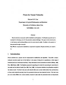
Fig. 7 Four graphical representations of a bag of tuples. In (a) and (b), a node stands for the bag and the other nodes denote the tuples. There may be edges directed from the bag to the tuples (a) but also edges in the opposite direction may be used (b). In (c) and (d), the bag is not represented and the tuples arranged in a sequence (c) or all connected (d).

each tuple (the first one). The presence of useless attributes makes more difficult the task of the relational learner, that has to single out the useful data while it is capturing the target function. For each bag, its dimension was defined by a random integer number generator using a uniform probability distribution in the range [5, 10]. In order to avoid biases in the results, the construction of the tuples consisted in two steps: first, the aggregation result was defined by a uniform probability distribution; then, a set of tuples that produced or approximated the expected result was generated by a pseudo–random procedure. Such a procedure depended on the particular aggregation function for the production of the first field, whereas the useless fields

30


were always assigned random values uniformly distributed in [−0.8, 0.8]. Thus, for the maximum function, the first field of each tuple contained random values smaller than the defined maximum, except for one tuple, which was forced to contain the exact result. For the sum, the tuples were recursively generated and, at each step, the first field was assigned a random value smaller than the difference between the current sum of the bag and the expected result; the last tuple was set so that the sum of the bag is the expected one. For the average, the first field was generated using a uniform distribution centered around the fixed average. The median dataset was generated in a similar way, but with the median instead of the average. Each bag was considered correctly predicted if the output of the network was within ±0.1 with respect to the target. Results have been averaged over three runs for each function. In each run, the dataset contained 500 bags: 300 in the training set, 100 in validation set and 100 in test set. Moreover, the number of epochs was 1000. The experimentation consisted of two parts. In an initial experiment, two basic RelNN and GNN models were tested; then several variations of those models were evaluated to measure the effect on the performance of the model parameters and of the data representation. The configuration of the basic models is:

– State dimension is 5 for both GNNs and RelNNs; – The GNN transition function hw and the GNN and RelNN output function gw are networks with one hidden layer, 5 hidden neurons, hyperbolic tangent


31

activation function in the hidden neurons and linear activation function in the output neurons; – In RelNN the transition function is implemented by a recurrent network rw with 5 locally recurrent neurons using the hyperbolic tangent activation function; – The weights are shared among all the nodes both in GNNs and in RelNNs15 – Bags of tuples are represented as in Fig. 7(a)16 . This configuration was chosen, by a preliminary experimentation, among those achieving the best performances and allowing a simple comparison of the models. However, the purpose was not that of measuring the maximal performance, so that an exhaustive experimentation was not carried out. Table 1 shows the results obtained by GNNs and RelNNs in the base experiment. Notice that the performance achieved by the two connectionist models varies largely according to the considered aggregation function. This variance partially depends on the general difficulty of neural networks to approximate some functions. For example, it is well know that even a simple feedforward neural network can approximate more easily a function that counts or sums the input values, than a function that computes the maximum. Actually, feedforward neural networks having just one hidden neuron can approximate up to any degree of precision the sum and the count 15

Notice that even if RelNNs have the capability to use different networks for different

types of nodes in representation (a) such a capability is not useful. In fact, the output function is evaluated only on the compound nodes and the transition functions only on the nodes representing the tuples. 16

It is worth mentioning that RelNNs can directly process such a representation without

a preliminary unfolding, since the graph in Fig. 7(a) is a tree.

32


maps [Gori et al., 1998]. On the other hand, the approximation of the maximum function requires a number of hidden units that depends on the desired precision. Similarly, the approximation of the average and the median is more difficult because they are composite functions: intuitively, the average requires to sum and to count the tuples, while the median needs to sort and count the tuples. On the other hand, the performance of the RelNN and the GNN models are very close on all the tasks. Such a fact is probably due to the simplicity of the considered problems and the simplicity of the data representation that does not highlight differences. GNN and RelNN have been also compared with a baseline approach in last row of Table 1. The baseline results were obtained by computing an optimal constant output on training set and using such a value as a response to every query. Such a comparison confirms that the two connectionist models learn to combine the information contained in the bags. More experiments have been carried out in order to evaluate how simple variations to the base configuration affect GNN performance. The first experiment compared different representations of a bag of tuples. More precisely, those depicted in Fig. 7 were considered. Representation (b) is equal to (a) with the difference that also the “belongs–to” relationship is used, i.e., there are edges going from the tuples to the sets. In (c), the tuples are arranged in a sequence where the edges link a tuple to the following one. Finally, in (d) the bag is not represented and all the tuples of a set are connected to each other by edges denoting the “belongs–to–the-same– bag” relationship. Both in (c) and (d), a tuple must be chosen to function as the


Count

Sum

33

Max

Model

GNN RelNN Baseline

Test

Train

Test

Train

100 [0]

100 [0]

100 [0]

100 [0]

Test

Train

48.3 [9.29] 61.3 [12.2]

99.0 [0.23] 99.5 [0.19] 99.8 [0.09] 99.9 [0.14] 45.1 [3.74] 63.0 [1.43] 16.7

16.7

16.0

16.0

Avg

10.8

11.0

Median

Model Test GNN RelNN Baseline

100 [0]

Train

Test

Train

99.8 [0.19] 84.3 [0.58] 87.3 [0.34]

99.0 [0.57] 99.7 [0.26] 80.9 [1.86] 89.32 [0.92] 18.4

19.0

31.0

31.2

Table 1 The accuracies (percentage) achieved with GNNs and RelNNs on the aggregation function experiment using the base configuration. The sample standard deviation is reported in square brackets.

supervised node: in our experiments, the selected tuple was the first that had been generated, randomly, during dataset creation. Moreover, also the ordering of the tuples in (c) is the one in which they were generated. Table 2 shows the achieved performances. Interestingly, the best result is obtained with representation (d), while one of the worst results is got by (c). Representation (d) is the one in which the graph diameter17 is minimal, whereas representation (c) has the maximal diameter. Thus, the difference in the performance is probably due to the long–term dependencies problem that afflicts also common recurrent 17

The diameter of a graph is the maximal distance between two nodes, where the distance

is defined as the minimal number of edges contained in path connecting the nodes.

34


Count

Sum

Max

Representation Test

Train

Test

Train

Base: Fig 7(a)

100 [0]

100 [0]

100 [0]

100 [0]

48.3 [9.29] 61.3 [12.17]

Fig 7(b)

100 [0]

100 [0]

100 [0]

99.3 [0]

58.3 [5.51] 82.1 [4.86]

Fig 7(c)

Test

Train

17.7 [0.58] 18.7 [0.34] 90.7 [8.33] 90.6 [6.77] 59.3 [19.63] 64.8 [16.37]

Fig 7(d)

100 [0]

100 [0]

100 [0]

no parent label

100 [0]

100 [0]

100 [0]

99.5 [0.25] 71 [6.93] 100 [0]

Avg

49.3 [9.29]

89.2 [8.34] 60.2[16]

Median

Representation Test Base: Fig 7(a) Fig 7(b)

100 [0]

Train

Test

Train

99.8 [0.19] 84.3 [0.58] 87.3 [0.34]

99.3 [1.15] 99.7 [0.58] 78.3 [0.58] 78.3 [2.18]

Fig 7(c)

97 [0]

96.6 [0.20]

80 [1]

85.9 [2.41]

Fig 7(d)

100 [0]

99.7 [0]

87 [2]

88.1 [0.79]

no parent label

100 [0]

100 [0]

82.7 [1.53] 88.3 [1]

Time (secs) Representation Test Train Base: Fig 7(a)

0.05 101.8

Fig 7(b)

0.09 150.4

Fig 7(c)

0.08 92.4

Fig 7(d)

0.28 499.2

no parent label 0.07 93.0 Table 2 The performance of the GNN model on the aggregation function benchmarks. The first row displays the result of the base configuration, while other rows show the performance of a number of variations: in rows 2–4, different representations of the bags of tuples; in row 5, the label of the parent is not used in transition function. Computation times (CPU elapsed times) are in seconds for each run (averaged on the five different aggregation functions) on a PC with a CPU Athlon 4600+. The average sample standard deviation is reported in square brackets.


35

networks [Bengio et al., 1994]. Intuitively, if the diameter of the graph is large, the encoding network behaves as a deep network and learning is difficult, since the derivatives of error w.r.t. the weights rapidly decrease when they are backpropagated. One may wonder whether the diameter of any input graph could be decreased by adding more edges. However, the edges cannot be chosen disregarding the fact that they have to represent useful information in the considered application domain. Moreover, the computation time is affected by the number of edges in the representation as confirmed by last column of Table 2. A difference between the standard versions of RelNNs and GNNs is in the information used by the transition networks: the label of the parent is adopted only by GNNs (compare Eq. (6) with Eq. (7)). This fact may be an advantage, because more information is used, or a disadvantage, because more parameters are needed. In another experiment, the label of the parent node was removed from the transition function commonly used by GNNs, i.e., hw (ln , xchi [n] , lchi [n] ) in Eq. (7) is replaced by hw (xchi [n] , lchi [n] ). However, the results on the base representation of Fig 7(a) do not single out a clear difference on the performance (see fifth row of Table 2), suggesting that here the two mentioned effects are balanced. Another set of experiments were dedicated to RelNNs, where the implementation of the transition function is varied. More precisely, three transition networks were evaluated: a locally recurrent neural network (the base configuration), a fully recurrent neural network and the sum of the outputs of a non–recurrent feedforward network adopting the GNN solution described by Eq. (7). Fully recurrent neural networks

36


have two layers: the input layer is fully connected to the output one, while the output neurons are also back connected to the input neurons. In locally recurrent networks, there is no feedback from output to input, but there is a back connection from each output neuron to the neuron itself. See [Back and Tsoi, 1994] for more details on those recurrent models. The parameters of the exploited network were those defined in the basic configuration, i.e., 5 neurons in the output layer, state dimension is 5, and 5 hidden neurons in the feedforward neural network. Table 3 shows that the best performance is achieved by the GNN “sum” transition function. In order to explain such a result, it is worth mentioning that, in theory, recurrent networks are a more general model that can implement transition functions which cannot be implemented by combining the outputs of a feedforward network18. However, recurrent networks rely on the order by which the inputs (the children, in this case) are processed. Moreover, recurrent networks are affected by the long– term dependencies problem [Bengio et al., 1994] that limits the performance on long sequences. Thus, when the number of children is large and/or the order is random and does not codify domain information, as in the current experiment, the “sum” transition function can be advantageous over the recurrent networks.

3.2 The mutagenesis dataset

The mutagenesis dataset [Debnath et al., 1991] is a small dataset, publicly available (e.g. in [mutagenesis, 1991]) and often used as a benchmark in the ILP literature [Lodhi and Muggleton, 2005]. It contains the descriptions of 230 nitroaromatic compounds 18

Fully recurrent networks have been proved to be universal approximators on sequences.


Count

37

Sum

Max

Representation Test

Train

Test

Train

Test

Train

Base: locally recurrent 99.0 [0.23] 99.5 [0.19] 99.8 [0.09] 99.9 [0.14] 45.08 [3.74] 63.0 [1.43] fully recurrent sum

99.0 [0.35] 99.2 [0.14] 99.7 [0.30] 99.8 [0.13] 57.8 [7.24] 72.2 [4.60] 99.9 [0.09]

100 [0]

99.8 [0.14] 99.8 [0.08] 78.1 [3.00] 84.1 [3.23]

Avg

Median

Representation Test

Train

Test

Train

Base: locally recurrent 99.0 [0.57] 99.7 [0.26] 80.9 [1.86] 89.3 [0.92] fully recurrent

96.0 [1.37] 98.0 [0.35] 75.7 [2.29] 88.6 [0.40]

sum

99.8 [0.17] 99.9 [0.04] 86.4 [1.22] 94.2 [0.64] Time (secs) Representation Test Train Base: locally recurrent

0.1

34.7

fully recurrent

0.1

37.4

sum

0.1

36.0

Table 3 The performance of the RelNN model on the aggregation function benchmarks. The results achieved by three different kind of transition functions are shown. Computation times (CPU elapsed times) are in seconds. Experiments were conducted on an Intel Core Duo E6850 CPU at 3 GHz.

that are common intermediate subproducts of many industrial chemical reactions. The goal of the benchmark consists of predicting which compounds are mutagenic on Salmonella typhimurium. In the original dataset, the value to be predicted was a real valued measure of the mutagenicity of each compound. In fact, in [Debnath et al., 1991] it is showed that 188 molecules out of 230 are amenable to a regression

38


analysis. This subset was therefore called “regression–friendly”, while the remaining 42 compounds were termed “regression–unfriendly”. However, as far as we know, the application considered in all the published papers is a classification problem where it has to be predicted whether a compound is mutagenic (mutagenicity is larger than one) or not (mutagenicity is smaller than one). The mutagenesis dataset can be obtained via anonymous FTP to ftp.comlab.ox.ac.uk in the directory pub/Packages/ILP/Datasets/mutagenesis. In this paper, we concentrate on the classification problem. GNNs and RelNNs were trained to output 1 when they are fed on a mutagenic compound and −1, when the pattern is not mutagenic. In the testing phase, a compound is predicted to be mutagenic or not according whether the model output is larger than 0 or not. Despite the fact that the dataset is quite small, it has been used intensively in the past ten year to evaluate statistical and relational learning techniques. For historical reasons, many authors have reported their results only on the “regression–friendly” part, that is often referred to as “the” mutagenesis dataset. Moreover, the comparison is complicated by the fact that many different features can be used in the prediction. Each compound is provided with four global features [Debnath et al., 1991]: two features are chemical measurements (C), namely LUMO, or lowest unoccupied molecule orbital and logP, or water/octanol partition coefficient19, while the other two features are pre-coded structural attributes (PS). Moreover, some features 19

Octanol is a fatty alcohol with eight carbon atoms that is immiscible with water.

Water/octanol partitioning, measured in logarithmic scale (LogP), is a relatively good approximation of the partitioning between the cytosol and lipid membranes of living systems.


39

describe properties of the single atoms: they include the atom type and the charge. The atom-bond structure is also given, which defines binary relationships between the atoms of each compound. Finally, the presence of functional groups (FG), e.g. methyl groups, have been used in some papers as higher level features. This last kind of features describes some properties of groups of atoms. In our experiments, the simplest representation, denoted by AB, includes the atom-bonds and the features of single atoms: the atom type and the charge. Moreover, atom types were represented by a one–hot coding20 of the 9 different types available in the dataset. All other features were denoted by the corresponding numerical values: the charge is a real and both C and PS are 2–dimensional vectors. The purpose of the experimentation on the mutagenesis dataset and, in the next section, on the biodegradability dataset is to compare, on well known benchmarks from the relational learning field, the performances of RelNNs and GNNs to each other and with respect to other models. Due to the large number of possible choices either in the representation of the data and in definition of the model parameters, an exhaustive comparison of all the possible solutions was not viable. Thus, in the following, we present the results obtained with a configuration that was chosen according both to a preliminary experimentation and some theoretical considerations. Such a preliminary study allowed us to define the most promising configurations for RelNNs and GNNs and the range of the parameters to be experimented. 20

A one–hot coding of a variable v that can assume a finite number of different values

v1 , . . . , va consists of a s–dimensional vector [t1 , . . . , ta ], such that if v = vi , then ti = 1 and tj = −1, for any j 6= 0, hold.

40


Two different graphical representations have been considered, that correspond to the cases where the data is represented by two tables (Compounds and Atoms) and one table only (Atoms), see Fig. 8. a) Each compound is denoted by a node that is labeled with the global features and is connected to other nodes representing the atoms that belong to the compound. The atom nodes are labeled with the type of the atom and are connected by edges to other nodes representing the bonded atoms. The attribute ”is mutagenic”, which has to be predicted, is naturally associated with the compound node. b) The compound is not represented. The nodes standing for atoms are connected as in (a), while their labels are extended with the global features. The supervised node can be any node: in practice, only the first node21 of each compound is supervised. The experimentation has been carried out using (a) for RelNNs and (b) for GNNs. Actually, the former representation is the more suited to represent the data for RelNNs, whereas the latter is suitable for GNNs. This difference is due to the fact that RelNNs use different neural networks for different relations, while GNNs do not. For this reason, RelNNs can gain an advantage from having two different relations while GNNs cannot. Some preliminary experimental results confirmed that RelNNs achieve the better performance with representation (a), whereas GNNs obtain the better performance with representation (b). 21

More precisely, the first node is the one corresponding to the first atom in the list of the

original dataset. As far we know, the ordering in the dataset has no particular meaning.


41

1

1

Supervised node Supervised node

3

2

3

2 5

r

5

4

4 7

7

6

6 10

10

8

8

9

(a)

9

(b)

Fig. 8 The graphical representations for the molecules of the mutagenesis dataset used for RelNNs (a) and for GNNs (b). In (a) the supervised node is a node representing the compound. In (b), the supervised node is one of the nodes representing the atoms.

Since representation (a) is cyclic, the graphs must be pre-processed using the unfolding procedure described in Algorithm 1. Figure 9 shows an example of the results of the unfolding of a compound.

r

4

Supervised node 2

r

3

1

1

2

2

3

3

4

(a)

2

4

4

2

3

(b)

Fig. 9 The unfolding tree (b) obtained by unfolding the compound (a) up to depth 3. For the sake of clarity, common substructures have not been merged.

Model configuration was as follows.

42


– The GNN transition function hw and the output function gw were implemented by feedforward neural networks with one hidden layer, hyperbolic tangent activation function in the hidden neurons and linear activation function in the output neurons. – In RelNNs, the transition function is implemented by a locally recurrent neural network rwn using hyperbolic tangent activations.

Following the experimental procedure commonly adopted on this benchmark, we used a 10-fold cross-validation scheme. The dataset L was randomly split into 10 folds L1 , . . . , L10 . For each i, an experiment was run using L \ Li for training and Li for testing. More precisely, L\Li was further randomly split into an training set and a validation set, where the validation set dimension equals the dimension of the test set, i.e., a 10% of the original dataset The results were averaged on all the folds and on 3 different runs. Validation sets were used to select the GNN and the RelNN parameter dimensions, i.e. the number of hidden neurons and the state dimension. Nine different configurations were evaluated by testing all the architectures that can be constructed by taking the number of hiddens22 in 2, 5, 10 and the state dimension in 2, 5, 10. Moreover, the RelNN model has been tested varying also the unfolding depth (in 1, 2, 3) and the transition function (choosing among a locally recurrent network (lrc), a fully recurrent network (frc) or the sum of the outputs of a feedforward network (sum)). The model architecture achieving the best result on the validation sets was 22

In order to keep small the number of experiments, only networks with the same number

of hiddens in the output function and the transition function were evaluated.


43

evaluated on test sets. More precisely, the best model is the one obtaining the lower error average over all the folds and all the 3 repetitions23 . The number of training epochs was chosen by two different criteria: (a) during training, the considered model was evaluated every 20 epochs on validation set and the epoch corresponding to best performance on validation set was considered the last epoch; (b) a large number of epochs (500 in this case) was chosen, where “large” is heuristically defined as a number several times larger than the number of epochs usually required by the learning algorithm to reach a point where the error does not decreases significantly on training set and on the validation set24 . In general, strategy (a) is preferable when a large validation set is available and it provides a precise prediction of the error on test set. On the other hand, the strategy (b) may be better provided that a too long learning time does not cause a loss of generalization capability due to the overfitting phenomenon. Table 4 shows the performances of GNNs and RelNNs on the two parts of the mutagenesis dataset and on the whole benchmark. The results indicate that, in our experimental setting, stopping criterion (b) (column “500 epochs”) is better than criterion (a) (column “Best on val.”) for GNNs, whereas the converse holds for RelNNs. In fact, in this case both the validation and the training sets are 23

It can be observed that such a procedure introduces a bias in the experiments, since the

patterns of a validation set are used also in test sets. On the other hand, the results aggregated by model allow to compare the different configurations. 24

It is worth to mention that for each experiment only one learning session is run for both

the strategies and that, in order to obtain a more fair comparison, the patterns originally assumed to the validation set has not been used to extend the training set in strategy (b).

44


probably too small: in GNN this gives rise to an early stop of the learning, whereas in RelNN an overfitting phenomenon is observed25. The different behaviour of the two models with respect to overfitting can be confirmed by observing the difference between the performances on training set and on test set, which is small for GNNs and large for RelNNs (see Table 5). The reason of the overfitting in RelNN, which has been not observed on the other datasets of this paper, has not been further investigated, even if it is probably due to the number of parameters, which is larger than in GNN, and to the (eventual) use of recurrent networks, whose performance depends on the sorting of children. Different sets of features for the labels were tested. More precisely, three cases were considered: only local properties and atom–bonds (denoted by AB)26 ; AB and chemical measurements (denoted by AB+C); AB+C and structural attributes (denoted by AB+C+PS)27 . The results in Table 4 indicate that GNNs and RelNNs can merge the global information with the local information. In particular, the best 25

It is worth to mention that the dimensions of the training set and the validation set have

been selected by heuristics and they have not been optimized. Probably, using different sizes for GNNs and RelNNs the performance can be improved. Also, by leave-one-out validation, we could enlarge the training set. However, those solutions have not been considered due to the long time required for running those experiments. 26

Atom-bonds define the connectivity between the atoms and are not explicitly stored in

labels. 27

Notice that the actual label content depends also on the representation. In representation

(b), the labels contain both the local and the global features (C, PS), whereas in representation (a), the local features are stored in the labels of the nodes standing for the atoms and the global features are stored in the labels of the nodes denoting the compounds.


45

performances are achieved when pure graph features AB are merged with node information C and C+PS.

Table 5 compares the performance of the models when different number of hidden neurons and different dimensions of the states are used. The table displays the performance on the whole mutagenesis dataset using the features AB+C+PS, similar results were obtained using only the friendly and the unfriendly parts of the benchmark and different sets of features. The results show that even if the number of hidden neurons and the state dimension affect the performance, the impact is not very large on the mutagenesis test set. Actually, this fact can be explained by observing that increasing the dimension of the models would allow to implement more “complex functions” on graphs. On the other hand, here such a capability is probably not exploited, because even if the ideal function that classifies correctly the compounds is complex, such a function is not precisely defined by the current training dataset that contains very few patterns. Thus, when the number of the parameters increase, only the performance on training set eventually improves, e.g., in RelNNs.

Moreover, differently from the experiments on the aggregation function problems, the best performances are achieved implementing the transition by recurrent networks (either locally recurrent (lrc) or fully recurrent (frc)) instead of a sum of the outputs of a feedforward network (sum). Such a difference may be due to the fact that the complexity of this problem allows to exploit the larger approximation capability of the recurrent networks.

46


Best architecture

Accuracy

Model Label content State Hidden Unf. Trans.

500

Best

dim.

dim.

epochs

on val.

depth type

Whole dataset GNN

AB

10

10

–

–

81.74 [2.42] 79.13 [1.99]

GNN

AB+C

5

2

–

–

88.12 [0.50] 85.51 [0.66]

GNN

AB+C+PS

10

2

–

–

87.54 [1.00] 86.38 [0.25]

RelNN

AB

2

10

2

sum 79.57 [2.01] 78.26 [0.64]

RelNN

AB+C

5

10

2

sum 77.10 [1.47] 79.57 [1.70]

RelNN

AB+C+PS

5

2

2

sum 80.87 [2.51] 83.04 [1.13]

Regression–friendly part GNN

AB

10

10

–

–

80.49 [0.81] 79.59 [0.63]

GNN

AB+C

2

5

–

–

94.83 [0.83] 93.61 [1.07]

GNN

AB+C+PS

2

2

–

–

95.92 [0.32] 93.06 [0.93]

RelNN

AB

2

10

2

sum 87.77 [2.48] 84.75 [1.82]

RelNN

AB+C

2

2

1

sum 87.77 [1.22] 88.30 [0.45]

RelNN

AB+C+PS

10

10

1

sum 88.30 [1.27] 91.49 [0.53]

Regression–unfriendly part GNN

AB

10

5

–

–

79.67 [2.75] 79.83 [1.44]

GNN

AB+C

2

10

–

–

95.83 [1.44] 89.83 [1.61]

GNN

AB+C+PS

2

10

–

–

95.83 [1.44] 94.33 [1.15]

RelNN

AB

2

2

2

sum 78.57 [7.72] 79.37 [2.71]

RelNN

AB+C

5

10

2

sum 70.63 [4.64] 80.95 [2.71]

RelNN

AB+C+PS

5

10

2

sum 73.02 [4.26] 80.16 [3.98]

Table 4 The performance of RelNNs and GNNs on mutagenesis benchmark. The columns display: the label content; the architecture that produces the best performance on validation set; the accuracies achieved at the end of the 500 training epochs and those achieved by the network that, during learning, has the best performance on validation set. The architecture is defined by the number of hidden neurons, the state dimension, the unfolding depth and the transition function, which can be a locally recurrent network (lrc), a fully recurrent network (frc) and the sum of the outputs of a feedforward network (sum).


47

On the other hand, using the feature set AB allows us to compare the representations of Figs 8(a) and 8(b) in a particular case. In fact, representations (a) and (b) differ both for the graph connectivity and for the label content. But, when AB is used, the atom labels have the same content both in (a) and (b). The performance of GNNs and RelNNs are closer in this case, which may suggest that the better GNN results may be due also to the different labels used by the two models. A review of the published results on the “regression–friendly” part can be found in [Lodhi and Muggleton, 2005], whereas [Ramon, 2002,Uwents and Blockeel, 2005] presents a selection of results using the full set of compounds. Tables 6, 7, 8 report the performance achieved by the state of the art techniques on the regression– friendly part, the regression–unfriendly part and the whole mutagenesis dataset, respectively. In order to simplify the comparison, those tables contain also a copy of the best results of RelNNs and GNNs. The comparison is not straightforward because different methods exploit different feature sets. However, if we focus on the absolute best performance of each method disregarding the used features, we can observe that GNNs outperform other methods on the regression-unfriendly part, while on the friendly part and on the whole dataset the results are close to the state of the art. RelNNs produce slightly lower results with respect to GNNs. On the other hand, if we take in consideration also the features, GNNs and RelNN performance is comparable or better than the other approaches except for the feature set AB. This fact can be explained by noticing that the capability of combining symbolic and sub–symbolic information is an important characteristic of the proposed models. Such a characteristic is less used

48

Werner Uwents et al. Architecture State Hidden Type dim. num

Train accuracy 500 epochs

Best on val.

Test accuracy 500 epochs

Best on val.

GNNs on whole dataset using AB+C+PS 2

2

89.84 [0.15] 86.90 [0.50] 87.97 [1.76] 87.25 [1.40]

2

5

90.96 [0.18] 87.67 [0.57] 88.70 [0.43] 87.10 [0.91]

2

10

91.57 [0.12] 87.68 [0.31] 88.70 [0.43] 86.38 [1.09]

5

2

90.17 [0.10] 87.63 [0.27] 87.39 [0.43] 85.80 [1.40]

5

5

91.07 [0.53] 88.22 [0.23] 88.41 [0.66] 86.81 [0.25]

5

10

91.72 [0.39] 87.54 [0.07] 87.97 [0.66] 86.09 [1.51]

10

2

89.82 [0.34] 87.48 [0.34] 87.54 [1.00] 86.38 [0.25]

10

5

90.94 [0.13] 87.41 [0.08] 88.99 [0.91] 87.10 [1.53]

10

10

91.56 [0.68] 88.08 [0.44] 89.13 [0.75] 86.23 [1.09]

RelNNs on whole dataset using AB+C+PS 2 2 2

2 2 2

lrc frc sum

89.62 89.64 86.81

83.37 87.54 82.54

81.01 81.30 78.70

80.72 81.45 81.01

2 2 2

5 5 5

lrc frc sum

94.28 95.49 92.36

83.71 84.24 83.24

76.67 79.13 79.13

81.30 82.17 80.72

2 2 2

10 10 10

lrc frc sum

96.88 98.24 94.71

82.64 85.92 85.63

76.38 74.78 77.25

80.58 79.86 78.99

5 5 5

2 2 2

lrc frc sum

91.18 89.75 85.43

82.14 86.41 83.55

80.87 80.87 78.26

80.29 83.04 77.97

5 5 5 5 5 5

5 5 5 10 10 10

lrc frc sum lrc frc sum

95.24 97.26 91.68 98.15 99.31 95.07

89.15 83.93 84.22 88.91 84.67 84.67

80.29 77.83 78.70 76.81 76.38 78.55

81.16 81.45 78.70 82.61 81.74 80.72

10 10 10

2 2 2

lrc frc sum

90.25 90.14 76.18

87.21 86.39 74.35

81.30 78.99 71.88

81.30 81.30 71.88

10 10 10

5 5 5

lrc frc sum

95.05 96.92 84.20

85.07 88.03 80.20

79.28 78.99 76.09

81.88 82.46 76.23

10 10 10

10 10 10

lrc frc sum

98.39 99.37 91.74

84.91 84.31 85.38

77.68 75.65 77.68

82.46 80.43 79.13

Table 5 The effect on the performance of the architecture. RelNNs and GNNs are evaluated on the whole mutagenesis dataset using the features AB+C+PS. The columns display: the architecture whose performance is displayed; the accuracies achieved at the end of the 500 training epochs and those achieved by the model that has the best performance on validation set. The architecture is defined by the number of hidden neurons, the state dimension, the unfolding depth and the transition function, which can be a locally recurrent network (lrc), a fully recurrent network (frc) and the sum of the outputs of a feedforward network (sum).


49

when the features set does not contain the global properties, so that, in this case, the models lose one of their advantages. Finally, it is interesting to note that whereas most of the approaches show a higher level of accuracy on the whole dataset than on the regression–unfriendly part, this is not true for our approaches. Such a behavior may suggest that the proposed connectionist models can capture particular characteristics of the dataset, which cannot be captured by other methods. Those characteristics, however, may not be homogeneously distributed in friendly and unfriendly parts. Such an odd distribution causes a difficulty in learning and gives rise to a decrease in the performance when both parts are used.

3.3 The biodegradability dataset

In this section, the experimentation carried out on the biodegradability dataset [Dzeroski, 1999, Dzeroski et al., 1999] is presented. Since the experimental procedure is very similar to that adopted for mutagenesis, in the following we only discuss the differences. The reader is referred to the previous section for the representation of the compounds, the model architectures and any other detail that is not explicitly reported here. The biodegradability dataset is very similar to the mutagenesis dataset. The aim is to predict the degree of biodegradability of 328 chemical compounds. The compounds are described by some global information, molecular weight and logP, and by the atoms and bonds that constitute them. For atoms and bonds, the type of atom or bond is given. This information gives a full description of the molecules,

50


Model

Label content

Reference

Accuracy

GNN

AB

80.49

GNN

AB+C

94.83

GNN

AB+C+PS

95.92

RelNN

AB

84.75

RelNN

AB+C

88.30

RelNN

AB+C+PS

91.49

RS

AB

[Lodhi and Muggleton, 2005]

88.9

RDBC

AB

[Kirsten, 2002]

84

1nn(dm )

AB

[Ramon, 2002]

83

FOIL

AB

[Quinlan and Cameron-Jones, 1993]

76

MFLOG

AB+C

[Kramer and De Raedt, 2001]

95.7

1nn(dm )

AB+C

[Ramon, 2002]

91

RDBC

AB+C

[Kirsten, 2002]

83

P-Progol

AB+C

[Srinivasan et al., 1994]

82.0

RS

AB+FG


89.9

Neural Networks

C+PS


89.0

RSD

AB+C+FG

[Krogel et al., 2003]

92.6

RELAGGS

AB+C+FG


88.0

P-Progol

AB+C+FG


88.0

SINUS

AB+C+FG


84.5

RS

AB+C+PS+FG


95.8

boosted-FOIL

not available

[Quinlan, 1996]

88.3

Table 6 A comparison of the performance of GNNs, RelNNs with other techniques on the regression–friendly part of the mutagenesis dataset.


Reference

51

Method

Label content

Accuracy

GNN

AB

79.67

GNN

AB+C

95.83

GNN

AB+C+PS

95.83

RelNN

AB

79.37

RelNN

AB+C

80.95

RelNN

AB+C+PS

80.16

TILDE

AB

[De Raedt and Blockeel, 1997]

85

RDBC

AB

[Kirsten, 2002]

79

1nn(dm )

AB

[Ramon, 2002]

72

TILDE

AB+C


79

RDBC

AB+C

[Kirsten, 2002]

79

1nn(dm )

AB+C

[Ramon, 2002]

72

Table 7 A comparison of the performance of GNNs, RelNNs with other techniques on the regression–unfriendly part of the mutagenesis dataset.

but in earlier experiments conducted on this dataset, extra descriptors were built. These extra descriptors include a vector of occurrences of functional groups and the counts of small substructures in the molecules. Thus five different features can be used for learning. Three of them are global values and are related to the whole molecule: P0 contains the molecular weight and logP; P1 consists of the counts of the different types of functional groups in the molecule; P2 consists of the counts of common substructures in the molecules. The other two features describe the atoms: R0 includes atom and bond type; R1 consists of background predicates on the functional groups and substructures. A

52


Method

Label content

Reference

Accuracy

GNN

AB

81.74

GNN

AB+C

88.12

GNN

AB+C+PS

87.54

RelNN

AB

78.26

RelNN

AB+C

79.57

RelNN

AB+C+PS

83.04

RDBC

AB

[Kirsten, 2002]

83

1nn(dm )

AB

[Ramon, 2002]

81

TILDE

AB


77

1nn(dm )

AB+C

[Ramon, 2002]

88

RDBC

AB+C

[Kirsten, 2002]

82

TILDE

AB+C


82

Table 8 A comparison of the performance of GNNs, RelNNs with other techniques on the whole mutagenesis dataset.

more detailed description of the information codified by R0, R1, P1 and P2 can be found in [Dzeroski et al., 1999],

In our experiments, atom and bond types were represented by one–hot coded vectors, whose length was 11 and 4. Other features were denoted by their respective values. Thus, P0 was a 2–dimensional vector, P1 and P2 were 30-dimensional sparse vectors.

For this dataset, researchers have studied both the corresponding regression problem, where the half life time has to be predicted and the classification problem,


53

where four categories were defined by common thresholds: chemicals that degrade fast, moderately fast, slowly, or are resistant. In the classification task, the output networks of RelNNs and GNNs had four output neurons corresponding to the biodegradability classes. A one–hot encoding schema was used to represent each class. The models were trained, by minimization of the common square error function, to return the vector that represents the class to which the processed molecule belongs to. In the testing phase, the class predicted by RelNNs and GNNs is the one corresponding to the largest output. The performance was measured by accuracy, i.e., the percentage of the correctly classified compounds, and by accuracy up to one error (accuracy ±1), which consists of the percentage of examples whose classification is at most one class up or down from the correct classification. For instance, a molecule that belongs to the class fast and is classified as moderately fast, still counts as correctly classified in accuracy ±1. In the regression task, the RelNN and GNN models, which had only one output, were trained using a real value denoting the degree of biodegradability. Similarly to the original paper [Dzeroski et al., 1999], the performance was evaluated using the correlation score between the output of the model and the target to be predicted. Table 9 displays the performance on the biodegradability dataset. The best overall result, both on the classification and the regression tasks, was obtained by GNNs with input R0+P0. In most of the input configurations, GNNs outperform RelNNs, except on regression task when all the features R0+P0+P1+P2 are used. Interestingly, the performance of both models is maximal when an intermediate configuration is used between the shortest input R0 and the longest R0+P0+P1+P2.

54


Such a fact can be explained by observing that a larger set of features requires a larger number of parameters and makes the networks more prone to fail in generalization and to have overfitting problems. It is also also interesting to notice that the performance of the models is high even without any preprocessed input feature, i.e., using R0, which includes only the graph connectivity and the bond and atom types. Moreover, differently from the experiments on the mutagenesis, the stopping criterion based on a large number of epochs and the criterion based on validation set achieve close performances. The only exception occurs for GNN accuracy on the classification task: in this case the former criterion clearly outperforms the latter. Notice that, even on the same task, observing the accuracy ±1, we cannot identify a method that is clearly preferable. This event may be explained observing that the square error function used during training tends to directly increase the accuracy, whereas the impact on accuracy ±1 is an expected consequence. Such a difference may indirectly changes the performance of the two stopping criteria. Table 10 illustrates the effect of using different numbers of hidden neurons and state dimensions28. It can be noticed that distance between the accuracy on the training set and the accuracy on the test set increases in GNNs when a larger number of parameters are employed. Such a behaviour confirms the presence of 28

For sake of brevity, the table shows only the performance on the classification task using

the features R0+P0, which is a case in the middle between the minimal number of features in R0 and the maximal in R0+P0+P1+P2. Moreover, for RelNNs, only the “sum” transition function is considered. However, the other cases showed similar results with respect to the goal of analyzing the effect of the number of hiddens and of state dimension.


55

Regression task Best architecture Model Label content State Hidden Unf. dim.

num

depth

Correlation

Trans.

500

Best

type

epochs

on val.

GNN

R0

10

10

0.6023 [0.0137] 0.6035 [0.0149]

GNN

R0+P0

5

10

0.6823 [0.0056] 0.6822 [0.0049]

2

10

RelNN

GNN R0+P0+P1+P2 R0

5

5

2

sum

0.6521 [0.0186] 0.6304 [0.0140]

RelNN

R0+P0

2

5

2

sum

0.6516 [0.0203] 0.6499 [0.0210]

RelNN

R0+P0+P1

5

2

2

lrc

0.6066 [0.0238] 0.6268 [0.0237]

RelNN

R0+P0+P2

5

5

1

lrc

0.5619 [0.0427] 0.6417 [0.0120]

2

5

1

frc

0.5287 [0.0244] 0.6729 [0.0213]

RelNN R0+P0+P1+P2

0.4449 [0.0411] 0.4452 [0.0413]

Classification task Best architecture

Accuracy

Model Label content State Hidden Unf. Trans.

GNN

R0

depth

type

Acc. (±1)

500

Best

500

Best

epochs

on val.

epochs

on val.

dim.

num

2

10

52.60 [0.97] 45.01 [1.36] 89.42 [0.94] 89.01 [1.70]

GNN

R0+P0

5

10

58.34 [0.97] 53.66 [3.51] 92.96 [0.91] 91.65 [0.18]

GNN

R0+P0+P1

10

10

54.85 [1.31] 42.66 [0.63] 91.55 [2.45] 89.60 [1.33]

GNN

R0+P0+P2

2

10

53.31 [1.63] 41.68 [1.97] 88.60 [1.37] 91.34 [1.53]

GNN R0+P0+P1+P2

2

10

R0

5

2

2

lrc

39.33 [3.16] 40.00 [1.37] 87.87 [1.30] 92.26 [0.63]

RelNN

R0+P0

2

2

1

frc

43.23 [1.60] 43.60 [0.43] 91.95 [1.56] 92.99 [0.83]

RelNN

R0+P0+P1

2

5

1

lrc

52.01 [4.01] 50.73 [1.62] 91.04 [1.19] 92.01 [1.02]

RelNN

R0+P0+P2

5

5

2

frc

48.72 [2.43] 47.62 [1.47] 88.60 [1.02] 90.67 [0.88]

2

5

2

lrc

49.94 [1.77] 51.46 [2.09] 89.39 [2.19] 91.22 [0.85]

RelNN

RelNN R0+P0+P1+P2

51.09 [1.85] 41.17 [0.02] 87.38 [2.00] 88.32 [1.55]

Table 9 The performance of RelNNs and GNNs on the biodegradability regression task (at the top) and on the classification task (at the bottom). The performance is measured by the accuracy and the accuracy up to one error (Test acc. ±1), for the classification task, and by the correlation score, for the regression task.

56


an overfitting problem that does not allow to improve the performance with larger inputs. It is worth mentioning that the same phenomenon, which is not evident on the R0+P0, arises also in RelNNs when larger inputs are used. Tables 11,12 show the results achieved on the classification task and on the regression task, respectively, as published in the literature [Dzeroski et al., 1999]. Notice that R0, which contains the graph connectivity, is needed by GNNs and RelNNs and has been always used in our experiments, whereas such information is not useful or even misleading for most of the other methods, since R0 is partially and implicitly contained in the other features. The tables prove that the performance of our models is comparable to the other best results, but not better: GNNs achieve the second best performance on classification task accuracy and on regression task. The high results obtained by methods that do not exploit R0 suggests that the counts of functional groups and substructures are probably a good propositionalization of the relational data (graph connectivity), as already mentioned in [Dzeroski et al., 1999]. On the other hand, the relatively high performance obtained by the presented approaches using only R0 suggest that those methods can actually extract a large part of the information in P0, P1, P2, R1 directly from the original graph. .

4 Conclusions

In this paper, we described and studied two recently proposed connectionist methods for graph processing called Graph Neural Networks and Relational Neural Networks.


Architecture State Hidden dim.

num

Train accuracy

Test accuracy

57

Test acc. (±1)

500

Best

500

Best

500

Best

epochs

on val.

epochs

on val.

epochs

on val.

GNNs on the classification task using R0+P0 2

2

66.96 [0.24] 56.33 [1.52] 53.11 [1.79] 49.10 [2.18] 92.26 [1.25] 90.22 [1.21]

2

5

74.57 [0.68] 58.03 [2.60] 56.79 [0.46] 48.27 [1.08] 92.16 [0.36] 92.25 [0.17]

2

10

78.39 [1.00] 58.86 [4.67] 57.09 [0.16] 47.48 [3.55] 91.64 [0.35] 91.03 [0.98]

5

2

67.03 [0.74] 57.75 [0.53] 53.33 [2.51] 51.42 [0.35] 90.22 [0.31] 89.61 [1.05]

5

5

75.61 [0.33] 61.06 [2.42] 57.82 [1.37] 49.97 [1.53] 92.56 [1.37] 90.92 [1.57]

5

10

79.52 [0.35] 64.58 [3.75] 58.34 [0.97] 53.66 [3.51] 92.96 [0.91] 91.65 [0.18]

10

2

66.75 [1.10] 54.72 [2.15] 52.93 [0.49] 48.87 [0.75] 90.63 [0.46] 91.02 [0.45]

10

5

75.71 [0.54] 59.96 [0.74] 57.30 [1.70] 49.49 [3.50] 92.46 [0.76] 89.80 [1.84]

10

10

79.12 [0.29] 64.71 [3.93] 56.71 [0.80] 52.64 [4.28] 93.17 [0.87] 91.35 [0.45]

RelNNs on the classification task using R0+P0 2

2

50.79

45.43

43.23

43.60

91.95

92.99

2

5

61.71

46.10

41.16

42.50

88.29

93.66

2

10

69.43

47.33

42.87

43.29

86.28

91.95

5

2

51.49

46.33

43.60

43.54

91.71

93.66

5

5

62.82

46.06

42.68

43.96

87.80

93.23

5

10

73.40

45.56

39.02

42.50

85.85

93.05

10

2

52.23

46.18

42.56

42.93

92.62

93.60

10

5

65.71

47.93

44.39

43.17

88.66

92.99

10

10

78.82

46.62

39.09

41.71

85.67

92.68

Table 10 The effect on the performance of the number of hiddens and the state dimension. RelNNs and GNNs are evaluated on the classification task of biodegradability using R0+P0. The columns display: the number of hiddens and state dimension of the model whose performance is displayed; the accuracies achieved at the end of the 500 training epochs and those achieved by the model that has the best performance on validation set.

58


Models

Label content

Accuracy

Accuracy ±1

GNN

R0

52.60

89.42

GNN

R0+P0

58.34

92.96

GNN

R0+P0+P1

54.85

91.55

GNN

R0+P0+P2

53.31

88.60

GNN

R0+P0+P1+P2

51.09

87.38

RelNN

R0

35.57

85.47

RelNN

R0+P0

36.59

88.11

RelNN

R0+P0+P1

42.68

91.16

RelNN

R0+P0+P2

40.65

90.96

RelNN

R0+P0+P1+P2

44.11

89.02

C4.5

P0+P1

55.2

86.2

C4.5

P0+P2

56.9

82.4

RIPPER

P0+P1

52.6

89.8

RIPPER

P0+P2

57.6

93.9

M5’

P0+P1

53.8

94.5

M5’

P0+P2

59.8

94.7

FFOIL

P0+R0

53.0

88.7

ICL

P0+R1

55.7

92.6

SRT-C

P0+P1

50.8

87.5

SRT-C

P0+P1+R1

55.0

90.0

SRT-R

P0+P1

49.5

91.9

SRT-R

P0+P1+R1

51.6

92.8

TILDE-C

P0+R1

51.0

88.6

TILDE-C

P0+P1+R1

52.0

89.0

TILDE-R

P0+R1

52.6

94.0

TILDE-R

P0+P1+R1

52.4

93.9

Table 11 A comparison of the performance of GNNs and RelNN with other methods on the classification task of the biodegradability benchmark.


Models

Label content

Correlation

GNN

R0

0.6023

GNN

R0+P0

0.6823

GNN

R0+P0+P1+P2

0.4449

RelNN

R0

0.6511

RelNN

R0+P0

0.6329

RelNN

R0+P0+P1

0.6253

RelNN

R0+P0+P2

0.5228

RelNN

R0+P0+P1+P2

0.5515

M5’

P0+P1

0.666

M5’

P0+P2

0.693

SRT-R

P0+P1

0.580

SRT-R

P0+P1+R1

0.632

TILDE-R

P0+R1

0.622

TILDE-R

P0+P1+R1

0.623

59

Table 12 A comparison of the performance of GNNs and RelNN with other methods on the regression task of the biodegradability benchmark.

The methods were compared and experimentally evaluated on benchmarks commonly used in relational learning field of research. The results are promising and suggest that RelNNs and GNNs can be viable approaches for learning on relational data. In particular, on mutagenesis, the performance of RelNNs and GNNs equals and, in some cases, outperforms the state of the art. A larger experimentation of the proposed models is matter of future research. In particular, the fields of bioinformatics and image localization appear to provide applications where GNNs and RelNNs may be useful. Moreover, a number of

60


extensions of the models can be investigated. For example, it may be interesting to study how the models can cope with dynamic information, i.e., input graphs that change along time, or how they can deal with missing information, for instance, label fields that are not available, and how the missing information can be eventually predicted. Moreover, several studies, which have been already carried out for common feedforward networks, should be extended to GNNs and RelNNs. For instance, the concept of Vapnik-Chervonenkis dimension and the cases when learning without local minima is possible have not been investigated for the proposed neural models.

References [Almeida, 1990] Almeida, L. B. (1990). A learning rule for asynchronous perceptrons with feedback in a combinatorial environment, pages 102–111. IEEE Press, Piscataway, NJ, USA. [Back and Tsoi, 1994] Back, A. and Tsoi, A. C. (1994).

Locally recurrent globally

feedforward networks, a critical review of architectures. IEEE Transactions on Neural Networks, 5(3):229–239. [Baldi and Pollastri, 2004] Baldi, P. and Pollastri, G. (2004). The principled design of large-scale recursive neural network architectures-DAG-RNNs and the protein structure prediction problem. Journal of Machine Learning Research, 4:575–602. [Bengio et al., 1994] Bengio, Y., Frasconi, P., and Simard, P. (1994). Learning long–term dependencies with gradient descent is difficult. IEEE Transactions on Neural Networks, 5:157–166. Special Issue on Recurrent Neural Networks. [Bianchini et al., 2006] Bianchini, M., Gori, M., Sarti, L., and Scarselli, F. (2006). Recursive processing of cyclic graphs. IEEE Transactions on Neural Networks, 17(1):10– 18.


61

[Bianchini et al., 2001] Bianchini, M., Gori, M., and Scarselli, F. (2001).

Processing

directed acyclic graphs with recursive neural networks. IEEE Transactions on Neural Networks, 12(6):1464–1470. [Bianchini et al., 2005] Bianchini, M., Maggini, M., Sarti, L., and Scarselli, F. (2005). Recursive neural networks for processing graphs with labelled edges: Theory and applications. Neural Networks - Special Issue on Neural Networks and Kernel Methods for Structured Domains, 18(8):1040–1050. [Bianchini et al., 2003] Bianchini, M., Mazzoni, P., Sarti, L., and Scarselli, F. (2003). Face localization with recursive neural networks. In Apolloni, B., Marinaro, M., and Tagliaferri, R., editors, Proceedings of WIRN03, volume 2859 of Lecture Notes in Computer Science, pages 99–105. Springer-Verlag. [Blockeel and Bruynooghe, 2003] Blockeel, H. and Bruynooghe, M. (2003). Aggregation versus selection bias, and relational neural networks.

In IJCAI-2003 Workshop on

Learning Statistical Models from Relational Data, SRL-2003, volume 11. [Bloehdorn and Blohm, 2006] Bloehdorn, S. and Blohm, S. (2006). A self organizing map for relation extraction from wikipedia using structured data representations. In Proceedings of the International Workshop on Intelligent Information Access, IIIA-2006. Springer-Verlag. [Brin and Page, 1998] Brin, S. and Page, L. (1998).

The anatomy of a large–scale

hypertextual Web search engine. Computer Networks and ISDN Systems, 30(1-7):107– 117. [Chang et al., 2000] Chang, H., Cohn, D., and K., M. A. (2000). customized authority lists.

Learning to create

In Proceedings of the 17th International Conference on

Machine Learning, ICML ’00, pages 127–134. Morgan Kaufmann. [Chapelle et al., 2006] Chapelle, O., Schölkopf, B., and Zien, A., editors (2006). SemiSupervised Learning. MIT Press, Cambridge, MA.

62


[De Raedt and Blockeel, 1997] De Raedt, L. and Blockeel, H. (1997). decision trees for clustering.

Using logical

In Proceedings of the 7th International Workshop on

Inductive Logic Programming ILP-97, volume 1297 of Lecture Notes in Artificial Intelligence, pages 133–141. Springer-Verlag. [Debnath et al., 1991] Debnath, A., Lopex de Compandre, R., Debnath, G., Schusterman, A., and Hansch, C. (1991).

Structure-activity relationship of mutagenic aromatic

and heteroaromatic nitro compounds. correlation with molecular orbital energies and hydrophobicity. Journal of Medicinal Chemistry, 34(2):786–797. [Di Massa et al., 2006] Di Massa, V., Monfardini, G., Sarti, L., Scarselli, F., Maggini, M., and Gori, M. (2006). A comparison between recursive neural networks and graph neural networks. In International Joint Conference on Neural Networks, pages 778–785. [Dzeroski, 1999] Dzeroski, S. (1999).

Biodegradability dataset, info at http://www-

ai.ijs.si/ ilpnet2/apps/pbiodeg.html. [Dzeroski et al., 1999] Dzeroski, S., Blockeel, H., Kompare, B., Kramer, S., Pfahringer, B., and Van Laer, W. (1999). Experiments in predicting biodegradability. Proceedings of the 9th International Workshop on Inductive Logic Programming, ILP-99, 1634:80–91. [Francesconi et al., 1998] Francesconi, E., Frasconi, P., Gori, M., Marinai, S., Sheng, J., Soda, G., and Sperduti, A. (1998). Logo recognition by recursive neural networks. In Tombre, K. and Chhabra, A. K., editors, GREC ’97: Selected Papers from the Second International Workshop on Graphics Recognition, Algorithms and Systems, pages 104– 117. Springer-Verlag. [Frasconi et al., 1998] Frasconi, P., Gori, M., and Sperduti, A. (1998).

A general

framework for adaptive processing of data structures. IEEE Transactions on Neural Networks, 9(5):768–786. [Gärtner, 2003] Gärtner, T. (2003). Kernel-based learning in multi-relational data mining. ACM SIGKDD Explorations, 5(1):49–58.


63

[Gärtner et al., 2004] Gärtner, T., Lloyd, J., and Flach, P. (2004). Kernels and distances for structured data. Machine Learning, 57(3):205–232. [Getoor and Taskar, 2007] Getoor, L. and Taskar, B. (2007). Introduction to Statistical Relational Learning. Mit Press. [Goller, 1997] Goller, C. (1997). A connectionist approach for learning search control heuristics for automated deduction systems.

PhD thesis, Technische Universit at

M unchen. [Goller and Küchler, 1996] Goller, C. and Küchler, A. (1996). Learning task-dependent distributed representations by backpropagation through structure. IEEE Transactions on Neural Networks, 1:347–352. [Gori et al., 2005] Gori, M., Monfardini, G., and Scarselli, F. (2005). A new model for learning in graph domains. In Proceedings International Joint Conference on Neural Networks (IJCNN2005), volume 2, pages 729–734. [Gori et al., 1998] Gori, M., Scarselli, F., and Tsoi, A. C. (1998). On the closure of set of functions that can be realized by a multilayer perceptron. IEEE Transactions on Neural Networks, 9(6):1086–1098. [Goulon-Sigwalt-Abram et al., 2005] Goulon-Sigwalt-Abram, Dreyfus, G. (2005).

A.,

Duprat,

A.,

and

From hopfield nets to recursive networks to graph machines:

numerical machine learning for structured data.

Theoretical Computer Science,

344(2-3):298–334. [Hagenbuchner et al., 2005] Hagenbuchner, M., Sperduti, A., and Tsoi, A. (2005). Contextual self-organizing maps for structured domains. In Proceedings of the Workshop on Relational Machine Learning, 16th European Conference on Machine Learning ECML 2005, volume 3720 of Lecture Notes in Computer Science, pages pp. 46–55. Springer. [Hagenbuchner et al., 2003] Hagenbuchner, M., Sperduti, A., and Tsoi, A. C. (2003). A self-organizing map for adaptive processing of structured data. IEEE Transactions on

64


Neural Networks, 14(3):491–505. [Hagenbuchner et al., 2009] Hagenbuchner, M., Sperduti, A., and Tsoi, A. C. (2009). Graph self-organizing maps for cyclic and unbounded graphs. Neurocomputation, 72(79):1419–1430. [Hagenbuchner et al., 2006] Hagenbuchner, M., Sperduti, A., Tsoi A. C., Trentini, F., Scarselli, F., and Gori, M. (2006). Clustering XML documents using self-organizing maps for structures. In Advances in XML Information Retrieval and Evaluation, volume 3977 of Lecture Notes in Computer Science, pages 481–496. Springer Berlin/Heidelber. [Hammer, 1999] Hammer, B. (1999). Approximation capabilities of folding networks. In Caudill, M. and Butler, C., editors, Proceedings of the 7th European Symposium on Artificial Neural Networks, ESANN 1999, pages 33–38. [Hammer and Jain, 2004] Hammer, B. and Jain, J. (2004).

Neural methods for non-

standard data. In M.Verleysen, editor, Proceedings of the 12th European Symposium on Artificial Neural Networks, ESANN 2004, pages 281–292. D-side publications. [Hammer et al., 2004a] Hammer, B., Micheli, A., Sperduti, A., and Strickert, M. (2004a). A general framework for unsupervised processing of structured data. Neurocomputing, 57:3–35. [Hammer et al., 2004b] Hammer, B., Micheli, A., Sperduti, A., and Strickert, M. (2004b). Recursive self-organizing network models. Neural Networks, 17(8-9):1061–1085. [Haykin, 1994] Haykin, S. (1994).

Neural Networks: A Comprehensive Foundation.

Prentice Hall, New York. [Jensen, 1996] Jensen, F. V. (1996). Introduction to Bayesian networks. Springer-Verlag. [Khamsi, 2001] Khamsi, M. A. (2001). An Introduction to Metric Spaces and Fixed Point Theory. John Wiley & Sons Inc. [Kirsten, 2002] Kirsten, M. (2002). Multirelational Distance-Based Clustering. PhD thesis, School of Computer Science, Otto-von-Guericke University, Magdeburg,


65

Germany. [Kleinberg, 1999] Kleinberg, J. (1999).

Authoritative sources in a hyperlinked

environment. Journal of the ACM, 46(5):604–632. [Kondor and Lafferty, 2002] Kondor, R. and Lafferty, J. (2002).

Diffusion kernels on

graphs and other discrete structures. In Sammut, C. and Hoffmann, A. G., editors, Proceedings of the 19th International Conference on Machine Learning, ICML 2002, pages 315–322. Morgan Kaufmann Publishers Inc. [Krahmer et al., 2003] Krahmer, E., Erk, S., and Verleg, A. (2003).

Graph-based

generation of referring expressions. Computational Linguistics, 29(1):53–72. [Kramer and De Raedt, 2001] Kramer, S. and De Raedt, L. (2001). Feature Construction with Version Spaces for Biochemical Applications.

In Proceedings of the 18th

International Conference on Machine Learning, ICML 2001, pages 258–265, San Francisco, CA, USA. Morgan Kaufmann Publishers Inc. [Krogel et al., 2003] Krogel, M., Rawles, S., Zelezny, F., Flach, P., Lavrac, N., and Wrobel, S. (2003). Comparative evaluation of approaches to propositionalization. In Proceedings of the 13th International Conference on Inductive Logic Programming, ILP 2003, volume 2835 of Lecture Notes in Computer Science, pages 197–214. Springer. [Lafferty et al., 2001] Lafferty, J., McCallum, A., and Pereira, F. (2001).

Conditional

random fields: Probabilistic models for segmenting and labeling sequence data.

In

Proceedings of 18th International Conference on Machine Learning. [Lodhi and Muggleton, 2005] Lodhi, H. and Muggleton, S. H. (2005). Is Mutagenesis still challenging? In Proceedings of the 15th International Conference on Inductive Logic Programming, ILP 2005, Late-Breaking Papers, pages 35–40. MIT Press. [McClelland et al., 1986] McClelland, J., Rumelhart, D., and the PDP Research Group (1986). Parallel Distributed Processing: Explorations in the Microstructure of Cognition, volume 2. MIT Press, Cambridge.

66


[Micheli, 2009] Micheli, A. (2009). Neural network for graphs: a contextual constructive approach. IEEE Transactions on Neural Networks, 20(3):498–511. [Micheli et al., 2004] Micheli, A., Sona, D., and Sperduti, A. (2004).

Contextual

processing of structured data by recursive cascade correlation. IEEE Transactions on Neural Networks, 15(6):1396–1410. [Micheli et al., 2001] Micheli, A., Sperduti, A., Starita, A., and Bianucci, A. M. (2001). Analysis of the internal representations developed by Neural Networks for structures applied to Quantitative Structure-Activity Relationship studies of benzodiazepines. Journal of Chemical Information and Computer Sciences, 41(2):202–218. [Money and Pollastri, 2009] Money, C. and Pollastri, G. (2009). Beyond the twilight zone: Automated prediction of structural properties of protein by recursive neural networks and remote homology information. Proteins: Structure, Function, and Bioinformatics, 77(1):181–190. [Monfardini and Scarselli, 2004] Monfardini, The

Graph

Neural

Networks

toolbox,

G. freely

and

Scarselli,

available

for

F.

(2004).

download

at

http://airgroup.dii.unisi.it/projects/GraphNeuralNetwork/download.htm. [mutagenesis, 1991] mutagenesis (1991). Mutagenesis dataset, available for download at http://www.comlab.ox.ac.uk/activities/machinelearning/mutagenesis.html. [Newman, 2001] Newman, M. E. J. (2001). From the cover: The structure of scientific collaboration networks. Proceedings National Academy of Sciences, 98(2):404–409. [Pineda, 1987] Pineda, F. (1987). Generalization of back–propagation to recurrent neural networks. Physical Review Letters, 59:2229–2232. [Quinlan and Cameron-Jones, 1993] Quinlan, J. and Cameron-Jones, R. (1993). FOIL: A midterm report. Proceedings of the European Conference on Machine Learning, pages 3–20.


67

[Quinlan, 1996] Quinlan, J. R. (1996). Boosting first-order learning. In Arikawa, S. and Sharma, A., editors, Proceedings of the 7th International Workshop on Algorithmic Learning Theory, ALT 1996, volume 1160 of Lecture Notes in Computer Science, page 143. Springer. [Ramon, 2002] Ramon, J. (2002). Clustering and instance based learning in first order logic. PhD thesis, K.U. Leuven, Belgium. [Riedmiller and Braun, 1993] Riedmiller, M. and Braun, H. (1993). A direct adaptive method for faster backpropagation learning: the RPROP algorithm. In Proceedings of the IEEE International Conference on Neural Networks, volume 1, pages 586–591, San Francisco, CA, USA. [Rodriguez, 2001] Rodriguez, P. (2001). Simple recurrent networks learn context-free and context-sensitive languages by counting. Neural Computation, 13:2093–2118. [Scarselli et al., 2009a] Scarselli, F., Gori, M., Monfardini, G., Tsoi, A. C., and Hagenbuchner, M. (2009a). Computational capabilities of Graph Neural Networks. IEEE Transactions on Neural Networks, 20(1):81–102. [Scarselli et al., 2009b] Scarselli, F., Gori, M., Monfardini, G., Tsoi, A. C., and Hagenbuchner, M. (2009b). The Graph Neural Network model. IEEE Transactions on Neural Networks, 20(1):61–80. [Scarselli et al., 2005] Scarselli, F., Yong, S., Gori, M., Hagenbuchner, M., Tsoi, A., and Maggini, M. (2005). Graph Neural Networks for ranking web pages. In Proceedings of the 2005 IEEE/WIC/ACM Conference on Web Intelligence, WI2005, pages 666–672, Washington, DC, USA. IEEE Computer Society. [Sperduti, 1994] Sperduti, A. (1994). Labelling RAAM. Connection Science, 6(4):429– 459. [Sperduti and Starita, 1997] Sperduti, A. and Starita, A. (1997).

Supervised neural

networks for the classification of structures. IEEE Transactions on Neural Networks,

68


8(3):714–735. [Srinivasan et al., 1994] Srinivasan, A., Muggleton, S., King, R., and Sternberg, M. (1994). Mutagenesis: ILP experiments in a non-determinate biological domain. In Wrobel, S., editor, Proceedings of the 4th International Workshop on Inductive Logic Programming. ILP 1994, volume 237 of GMD-Studien, pages 217–232. Gesellschaft für Mathematik und Datenverarbeitung MBH. [Sturt et al., 2003] Sturt, P., Costa, F., Lombardo, V., and Frasconi, V. (2003). Learning first-pass structural attachment preferences with dynamic grammars and recursive neural networks. Cognition, 88(2):133–169. [Tsoi et al., 2006] Tsoi, A. C., Hagenbuchner, M., and Scarselli, F. (2006). Computing customized page ranks. ACM Transactions on Internet Technology, 6(4):381–414. [Tsoi et al., 2003] Tsoi, A. C., Morini, G., Scarselli, F., Hagenbuchner, M., and Maggini, M. (2003). Adaptive ranking of web pages. In Proceedings of the 12th International Conference on World Wide Web, WWW 2003, New York, NY, USA. ACM. [Uwents and Blockeel, 2005] Uwents, W. and Blockeel, H. (2005). Classifying relational data with neural networks. In Proceedings of the 15th International Conference on Inductive Logic Programming, ILP 2005, volume 3625 of Lecture Notes in Computer Science, pages 384–396. Springer. [Vapnik, 1998] Vapnik, V. N. (1998). Statistical Learning Theory. Wiley. [Wang et al., 2002] Wang, Z., Hagenbuchner, M., Tsoi, A., and Cho, S.Y. Chi, Z. (2002). Image classification with structured self-organization map. In Proceedings of the 2002 International Joint Conference on Neural Networks, IJCNN 2002, volume 2, pages 1918– 1923, Piscataway, NJ, USA. IEEE Press. [Werbos, 1990] Werbos, P. (1990). Backpropagation through time: what it does and how to do it. Proceedings of the IEEE, 78(10):1550–1560.


69

[Yong et al., 2006] Yong, S., Hagenbuchner, M., Scarselli, F., Tsoi, A. C., and Gori, M. (2006). Document mining using Graph Neural Networks. In Fuhr, N., Lalmas, M., and Trotman, A., editors, Proceedings of the 5th International Workshop of the Initiative for the Evaluation of XML Retrieval, INEX 2006, Revised and Selected Papers, volume 4518 of Lecture Notes in Computer Science, pages 458–472. Springer.

Neural networks for relational learning: An experimental ... - CiteSeerX

Neural networks for relational learning: An experimental ... - CiteSeerX

Suggest Documents

Randomized Neural Networks for Learning Stochastic ... - CiteSeerX

Neural Networks Learning transform invariant object ... - CiteSeerX

Incremental Backpropagation Learning Networks - Neural ... - CiteSeerX

Incremental Backpropagation Learning Networks - Neural ... - CiteSeerX

Priors for Neural Networks - CiteSeerX

Dependency Networks for Relational Data - CiteSeerX

an incremental learning algorithm for supervised neural networks

Self-organizing neural networks for learning air combat ... - CiteSeerX

WPA3-6 Learning Algorithms for Cellular Neural Networks - CiteSeerX

Ml-rbf: RBF Neural Networks for Multi-Label Learning - CiteSeerX

Neural Networks Incremental learning for Î½-Support ... - CiteSeerX

A Least-Squares Learning for Block-based Neural Networks - CiteSeerX

Ml-rbf: RBF Neural Networks for Multi-Label Learning - CiteSeerX

Learning Methods for Dynamic Neural Networks - IEICE

Deep neural networks for learning classification ...

Unsupervised Learning Procedures for Neural Networks Suzanna

Learning Opposites Using Neural Networks

Neural Networks and Statistical Learning

Neural Networks Learning Relative Distances

Neural Networks and Statistical Learning

Neural Networks and Statistical Learning

Learning Polynomials with Neural Networks

Neural Networks and Statistical Learning

Fast Learning of Relational Dependency Networks