Morgan Stanley index Germany. 6. Dow Jones industrial index. 7. DM-USD exchange rate. 8. US treasury bonds. 9 gold price in DM. 10. Nikkei index Japan. 11.
Apr 15, 2015 - ... in Big Networks. Quan-Lin Li. School of Economics and Management Sciences ...... Laboratory, Christ's College, University of Cambridge. 22 ...
14. Dynamical Nonlinear Neural Networks with. Perturbations Modeling and Global Robust Stability. Analysis. Gamal A. Elnashar. Automatic Control Center.
cost-sensitive classification without going through a probability estima- ... *Department of Computer Science, University of Maryland, College Park, MD 20783. 1 ...
a standard 0/1-loss structured classifier to estimate class conditional prob- abilities ..... For the cost-sensitive version of the structured classification problem, in addition to (G, Ψ) .... Note that the summations in the final expression are li
Most of the material in the book is taken from a series of papers [ 11 ... of Chapter 1 deals with the existence and uniqueness of solutions of abstract networks ...
Apr 12, 2013 - Angelo Antociâ ... e-mail: [email protected]. .... neration Lt · Wt is saved and entirely invested in productive capital Kt+1 (i.e.. Kt+1 = Lt ...
Jean-Pierre Nadal, Nicolas Brunel. Laboratoire de Physique Statistique de l'E.N.S.*. Ecole Normale Sup erieure. 24, rue Lhomond, F-75231 Paris Cedex 05, ...
Ivana Komunjer, Alisdair McKay, Juan Rubio-RamÃrez, Andres Santos, ..... degree NewtonâCotes-type formulas, or the ClenshawâCurtis quadrature (see Davis and ... Let pkn(j) be the probability that ykt = ¯ykn conditional on being in state j.
A Markov Logic Network (MLN) is a set of pairs. (F i. , w i. ) where. F i is a formula in first-order logic. w ... A dis
An Experiment Using MLNs to Extract Ontology Concepts from Text power of relational ..... Cunningham, H.: GATE, a general architecture for text engineering.
take in input graphs and trees directly, embedding the relationships between nodes into the ...... by feedforward neural networks with one hidden layer, hyperbolic tangent activation ...... with Version Spaces for Biochemical Applications.
Nov 7, 2007 - University of Houston. 01 December ... J.E.Cairnes Graduate School of Business and Public Policy ... and are often associated with the existence of auto-correlations that describe ...... Nonequilibrium Statistical Mechanics.
variational methods ; G ibb s sampling. 1 Introduction. Hidden Markov models (
HMMs) are a ubiquitous tool for modelling time series data. They are used in.
Nov 29, 2018 - ing and the application of convolutional neural networks (CNN). .... that are involved in the update process are interpretable and can be.
surveillance and traffic monitoring. The common ground of ... We propose the use of Relational Dynamic Bayesian Networks, an extension of Dynamic Bayesian ...
Ï â P(E). Nonlinear Markov kernels (see [FeynmanâKac Formulae: Genealogical and Interacting Par- ..... [(1 â ϵ)K(xn,dxn+1) + ϵ (SY .... global Lipschitz continuity results for μ â¦â Qμ, which, together with the result above, will allow.
Online Max-Margin Weight Learning with Markov Logic Networks. Tuyen N. Huynh and Raymond J. Mooney. Department of Computer Science. The University ...
Context interpretation and context-based reasoning have been shown to be key ... if car X exits but not car Y , the belief they are traveling together is greatly decreased: .... Probabilistic graphical models are graphs in which nodes represent rando
Jul 18, 2012 - Keywords Markov logic networks · Structure learning · Bayesian ... data are very common in practice, an important goal is to extend machine.
problem: learning the structure of an MLN that models the distribution of discrete descriptive attributes on medium to large datasets, given the links between ...
Aug 8, 2017 - the distributions of variables, we use the non-parametric estimators from previous ..... matrix from the G-Wishart distribution given this graph.
OCL has been mapped in relational calculus. In [17], a ... (CSG) â the constructs to represent any context of business analysis. A set of vertices of ..... [6] Karl Hahn, Carsten Sapia, Markus Blaschka, .... (2005), http://download.oracle.com/docs/
bilistic computations are well-understood in isolation, their combination is chal- lenging. .... And third, we support reasoning with what are called shift couplings ...
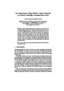
The two tables are shown on the left. On the right ... The situation is depicted in Figure 1. ... rules are automatically derived in a manner shortly described below. .... Using a Markov network and the BP algorithm corresponds to using probability.
Nonlinear Relational Markov Networks with an Application to the Game of Go Tapani Raiko Neural Networks Research Centre, Helsinki University of Technology, P.O.Box 5400, FI-02015 HUT, Espoo, FINLAND [email protected] Abstract. It would be useful to have a joint probabilistic model for a general relational database. Objects in a database can be related to each other by indices and they are described by a number of discrete and continuous attributes. Many models have been developed for relational discrete data, and for data with nonlinear dependencies between continuous values. This paper combines two of these methods, relational Markov networks and hierarchical nonlinear factor analysis, resulting in joining nonlinear models in a structure determined by the relations in the data. The experiments on collective regression in the board game go suggest that regression accuracy can be improved by taking into account both relations and nonlinearities.
1 Introduction Growing amount of data is collected every day in all fields of life. For the purpose of automatic analysis, prediction, denoising, classification etc. of data, a huge number of models have been created. It is natural that a specific model for a specific purpose works often the best, but still, a general method to handle any kind of data would be very useful. For instance, if an artificial brain has a large number of completely separate modules for different tasks, the interaction between the modules becomes difficult. Probabilistic modelling provides a well-grounded framework for data analysis. This paper describes a probabilistic model that can handle data with relations as well as discrete and continuous values with nonlinear dependencies. Terminology: Using Prolog notation, we write knows(alex, bob) for stating a fact that the knows relation holds between the objects alex and bob, that is, Alex knows Bob. The arity of the relation tells how many objects are involved. The knows relation is binary, that is, between two objects, but in general relations can be of any arity. The atom knows(alex, B) matches all the instances where the variable B represents an object known by Alex. In this paper, the terms are restricted to constants and variables, that is, compound terms such as thinks(A, knows(B, A)) are not considered. For every relation that is logically true, there are associated attributes x, say a class label or a vector of real numbers. The attributes x(knows(A, B)) describe how well A knows B and whether A likes or dislikes B. The attribute vector x(con(A)) describes what kind of a consumer the person A is. Given a relational database describing relationships between people and their consuming habits, we might study the dependencies that might be found. For instance, some people cloth like their idols, and nonsmokers tend to be
KNOWS who
whom how
Bob
CONSUMER who
Bob
consumer
consumer
smoker ...
Alex Bob
friend
Alex no
...
Bob
Carl
neighbour
Bob
no
...
Carl
Alex colleague
Carl
no
...
knows
knows knows
Alex
consumer knows
knows
Alex
Carl
consumer
consumer
knows
Carl
consumer
Fig. 1. Consider a relational database describing the relationships and consumer habits of three people. The two tables are shown on the left. On the right, the database is represented graphically, with the occurrences of the template (con(A), knows(A, B), con(B)) marked with ovals on the very right.
friends with nonsmokers. The modelling can be done for instance by finding all occurrences of the template (con(A), knows(A, B), con(B)) in the data and studying the distribution of the corresponding attributes. The situation is depicted in Figure 1. Bayesian networks[6] are popular statistical models based on a directed graph. The graph has to be acyclic, which is in line with the idea that the arrows represent causality: an occurrence cannot be its own cause. In relational generalisations of Bayesian networks [7], the graphical structure is determined by the data. Often it can be assumed that the data does not contain cycles, for instance in the case when the direction of the arrows is always from the past to the future. Sometimes the data has cycles, like in Figure 1. Markov networks [6], on the other hand, are based on undirected graphical models. A Markov network does not care whether A caused B or vice versa, it is interested only whether there is a dependency or not.
2 Model Description This section describes the models that are combined into nonlinear relational Markov networks. 2.1 Hierarchical Nonlinear Factor Analysis (HNFA) In (linear) factor analysis, continuous valued observation vectors x(t) are generated from unknown factors (or sources) s(t), a bias vector b, and noise n(t) by x(t) = As(t) + b + n(t). The factors and noise are assumed to be Gaussian and independent. The index t may represent time or the object of the observation. The mapping A, the factors, and parameters such as the noise variances are found using Bayesian learning. Factor analysis is close to principal component analysis (PCA). The unknown factors may represent some real phenomena, or they may just be auxillary variables for inducing a dependency between the observations. Hierarchical nonlinear factor analysis (HNFA) [11] generalises factor analysis by adding more layers of factors that form a multi-layer perceptron type of a network. In this paper, there are two layers of factors h and s, and the mappings are: h(t) = Bs(t) + b + nh (t) x(t) = Af [h(t)] + Cs(t) + a + nx (t) ,
(1) (2)
where the nonlinearity f (ξ) = exp(−ξ 2 ) operates on each element separately. HNFA can easily be implemented using the Bayes Blocks software library [10, 12]. The update rules are automatically derived in a manner shortly described below. The unknown variables θ (factors, mappings, and the parameters) are learned from data with variational Bayesian learning [4]. A parametric distribution q(θ) over the unknown variables θ is fitted to the true posterior distribution p(θ | X) where the matrix X contains all the observations x(t). The misfit is measured by Kullback-Leibler divergence D(· k ·). An additionalRterm − log p(X) is included to avoid calculation of the model evidence term p(X) = p(X, θ)dθ. The cost function is q(θ) C = D(q(θ) k p(θ|X)) − log p(X) = log , (3) p(X, θ) where h·i denotes the expectation over distribution q(θ). Note that since D(q k p) ≥ 0, it follows that the cost function provides a lower bound for the model evidence p(X) ≥ exp(−C). The posterior approximation q(θ) is chosen to be Gaussian with a diagonal covariance matrix. It is possible, though slightly impractical, to model also discrete values in HNFA by using the discrete variable with a soft-max prior [12]. In the binary case, the ith component of x(t) is left as a latent auxiliary variable, and an observed binary variable y(t) exp xi (t) is conditioned by p(y(t) = 1 | xi (t)) = 1+exp xi (t) . The general discrete case follows analogously requiring more than one auxiliary component of x(t). The experiments in Section 3 use a thousand copies of a binary variable having the same conditional probability. They can be united into one variable by multiplying its cost by one thousand. Observing 800 ones and 200 zeros corresponds to fixing the variable to a distribution of 0.8 times one and 0.2 times zero. 2.2 Relational Markov Networks (RMN) A relational Markov network (RMN) [9] is a model for data with relations and discrete attributes. It is specified by a set of clique templates C and corresponding potentials Φ. Using the example in the introduction, a model can be formed by defining a single clique template C = (con(A), knows(A, B), con(B)) and the corresponding potential φC over x(C) which is (a subset of) the concatenation of attribute vectors x(con(A)), x(knows(A, B)), and x(con(B)). Given a relational database, the RMN produces an unrolled Markov network over all the attributes X. The cliques c ∈ C(I) instantiated by a template CQshare the Qsame clique potential φC . The combined probabilistic model is p(X) = Z1 C∈C c∈C(I) φC (x(c)), where Z is a normalisation constant and C(I) contains all the instantiations of the template C. In general, a template can be any boolean formula over the relations. The general inference task is to compute the posterior distribution over all the variables X. The network induced by data can be very large and densely connected, so exact inference is often intractable [9]. The belief propagation (BP) algorithm [6] is guaranteed to converge to the correct marginal probabilities only for singly connected Markov networks, but it is used as a good approximation also in the loopy case. The learning task, or the estimation of the potentials Φ is done using the maximum a posteriori criterion. It requires an iterative algorithm alternating between updating the parameters of the potentials and running the inference algorithm on the unrolled Markov network.
2.3 Nonlinear Relational Markov Networks (NRMN) In nonlinear relational Markov networks (NRMN), the clique potentials are replaced by a probability density function for continuous values, in this case HNFA1 The combination of these two methods is not completely straightforward. For instance, marginalisation required by the BP algorithm is often difficult with nonlinear models. Also, algorithmic complexity needs to be considered, since the model will be quite demanding. One of the key points is to use probability densities p in place of potentials Φ. Then, overlapping templates give multiple probability functions for some variable and they are combined using the product-of-experts combination rule described below. Combination Rules: One of the non-trivialities in making relational extensions of probabilistic models is the so called combination rule [7]. When the structure of the graphical model is determined by the data, one cannot know in advance how many links there are for each node. One solution is to use combination rules such as the noisy-or. Combination rule transforms a number of probability functions into one. Noisy-or does not generalise well to continuous values, but two alternatives are introduced below. Using a Markov network and the BP algorithm corresponds to using probability densities as potentials and the maximum entropy combination rule. The probability densities pC (x(C)) are combined to form the joint probability distribution by maximising the entropy of p(X) given that all instantiations of pC (x(C)) coalesce with the corresponding marginals of p(X). For singly Q connected networks, this means that the joint Q distribution is p(X) = c pc (x(c))/ k pk (x(k)), where k runs over pairs of instantiations of templates and x(k) contains the shared attributes in those pairs. Marginalisation of nonlinear models cannot usually be done exactly and therefore one should be very careful with the denominator. Also, one should take care in handling loops. In the product-of-experts (PoE) combination rule, the logarithm of the probability density of each variable is the average of the logarithms of the probability functions that qQ Q the variable is included in: p(x) ∝ n C∈C c∈C(I) pC (x) for all x ∈ X, where only those n instantiated templates c that contain x, are considered. PoE is easy to implement in the variational Bayesian framework because the term in the cost function (3) can be split into familiar looking terms. Consider the combination of two probability functions p1 (x) and p2 (x) (that are assumed to be independent): E D E * + D q(x) + log log pq(x) (x) p (x) q(x) 1 2 log p . (4) = 2 p1 (x)p2 (x)
A characteristic of PoE is that implicit weighting happens in some sense automatically. When one of the experts gives a distribution with a large variance and another one with a small variance, the combination is close to the one with small variance. Inference in Loopy Networks: Inferring unobserved attributes in a database is in this case an iterative process which should end up in a cohesive whole. Information can traverse through multiple relations. 2 The basic element in the inference algorithm 1 2
One could also think in terms of e.g. a mixture model. In mixture of experts (MoE), it is enough when only one of the experts explains the data even if all the other disagree. The ignored experts will not pass information on. This explains why the author did not consider MoE as a combination rule.
of Bayes Blocks is the update of the posterior approximation q(·) of a single unknown variable, assuming the rest of the distribution fixed. The update is done such that the cost function (3) is minimised. One should note that when the distribution over the Markov blanket of a variable is fixed, the local update rules apply, regardless of any loops in the network. Therefore the use of local update rules is well founded, that is, local inference in a loopy network does not bring any additional heuristicity to the system. Also, since the inference is based on minimising a cost function, the convergence is guaranteed, unlike in the BP algorithm. Learning: The learning or parameter estimation problem is to find the probability functions associated with the given clique templates C. Now that we use probability functions instead of potentials, it is possible in some cases to separate the learning problem into parts. For each template C ∈ C, find the appropriate instantiations c ∈ C(I) and collect the associated attributes x(c) into a table. Learn a HNFA model for this table ignoring the underlying relations. This divide-and-conquer strategy makes learning comparatively fast, because all the interaction is avoided. There are some cases that forbid this. If the data contains missing values, they need to be inferred using the method in the previous paragraph. Also, it is possible to train experts cooperatively rather than separately [3]. Clique Templates: In data mining, so called frequent sets are often mined from binary data. Frequent sets are groups of binary variables that get the value 1 together often enough to be called frequent. The generalisation of this concept to continuous values could be called the interesting sets. An interesting set contains variables that have such strong mutual dependencies that the whole is considered interesting. The methodology of inductive logic programming could be applied to finding interesting clique templates. The definition of a measure for interestingness is left as future work. Note that the divide-and-conquer strategy described in the previous paragraph becomes even more important if one needs to consider different sets of templates. One can either learn a model for each template separately and then try combinations with the learned models, or try a combination of templates and learn cooperatively the models for them. Naturally the number of templates is much smaller than the number of combinations and thus the first option is computationally much cheaper. So what are meaningful candidates for clique templates? For instance, the template (con(A), con(B)) does not make much sense. Variables A and B are not related to each other, so when all pairs are considered, con(A) and con(B) are always independent and thus uninteresting by definition. In general, a template is uninteresting, if it can be split into two parts that do not share any variables. When considering large templates, the number of involved attributes grows large as well, which makes learning more involved. An interesting possibility is to make a hierarchical model. When a large template contains others as subtemplates, one can use the factors s in Eq. (1, 2) of the subtemplate as the attributes for the large template. The factors already capture the internal structure of the subtemplates and thus the probabilistic model of the large template needs only to concentrate on the structure between its subtemplates.
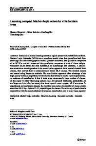
3 Experiments with the Game of Go Game of Go: Go is an ancient oriental board game. Two players, black and white, alternately place stones on the empty points of the board until they both pass. The standard board is 19 by 19 (i.e. the board has 19 lines by 19 lines), but 13-by-13 and 9-by-9 boards can also be used. The game starts with an empty board and ends when it is divided into black and white areas. The one who has the larger area wins. Stones of one colour form a block when they are 4-connected. Empty points that are 4-connected to a block are called its liberties. When a block loses its last liberty, it is removed from the board. After each move, surrounded opponent blocks are removed and only after that, it is checked whether the block of the played move has liberties or not. There are different rulesets that define more carefully what a “larger area” is, whether suicide is legal or not, and how infinite repetitions are forbidden. Computer Go: Of all games of skill, go is second only to chess in terms of research and programming efforts spent. While go programs have advanced considerably in the last 10-15 years, they can still be beaten easily by human players of moderate skill. [5] One of the reasons behind the difficulty of static board evaluation is the fact that there are stones on board that will eventually be captured, but not in near future. In many cases experienced go players can classify these dead stones with ease, but using a simple look-ahead to determine the status of stones is not always feasible since it might take dozens of moves to actually capture the stones. Experiment Setting: The goal of the experiments was to learn to determine the status of the stones without any lookahead. An example situation is given in Figure 2. The data was generated using a go-playing program called Go81 [8] set on level 1 and using randomness to have variability. By playing the game from the current position to the end a thousand times, one gets an estimate of who is going to own each point on the board. Information on the board states was saved to a relational database with two tables for learning an NRMN. The x(block(A)) contains the colour, the number of liberties, the size, distances from the edges, influence features in the spirit of [1], and finally the count of how many times the block survives in the 1000 possible futures. The ally(A, B) and enemy(A, B) contain a measure of strength of the connection between the blocks A and B estimated using similar influence features [1]. Only the pairs with a strong enough influence on each other (> 0.02) were included. One thousand 13-by-13 board positions after playing 2 to 60 moves were used for learning. Two clique templates, ((block(A), ally(A, B), block(B)) and an analogous one for enemy, were used. HNFA models were taught with 28 attributes of the two blocks and the pair. The dimensionality of the s layer was 8. The learning algorithm pruned the dimensionality of the h layer to 41 for allies and to 47 for enemies. The models were learned for 500 sweeps through the data. A linear factor analysis model was learned with the same data for comparison. A separate collection of 81 board positions with 1576 blocks was used for testing. The status of each block was now hidden from the model and only the other attributes were known. With inference in the network, the status were collectively regressed. As a comparison experiment, the inferences were also done separately, and combined only in the end. Inference required from four to thirty iterations to converge. As a postprocessing step, the regressed survival probabilities xˆ
Fig. 2. The leftmost subfigure shows the board of a go game in progress. In the middle, the expected owner of each point is visualised with the shade of grey. For instance, the two white stones in the upper right corner are very likely to be captured. The rightmost subfigure shows the blocks with their expected owner as the colour of the square. Pairs of related blocks are connected with a line which is dashed when the blocks are of opposing colours.
were modified with a simple three-parameter function x ˆnew = aˆ xb + c and the three parameters that gave the smallest error for each setting, were used. Results: The table below shows the root mean square (rms) errors for inferring the survival probabilities of the blocks in test cases. They can be compared to the standard deviation 0.2541 of the probabilities. rms error Linear Nonlinear Separate regression 0.2172 0.2052 Collective regression 0.2171 0.2037 As expected, nonlinear models were better than linear ones and collective regression was better than separate regression.
4 Discussion and Conclusion A traditional Markov network was applied for statically determining the status of the go board in [2]. Games played by people were used as data. Humans play the game better, but still, this approach has an important downside. The data contains only one possible future for each board position whereas a computer player can produce many possible futures. At the learning stage, all those futures can be used together for the computational price of one. Also, stones that are provably determined to be captured under optimal play (dead), might still be useful: By threathening to revive them, the player can gain elsewhere. When data is gathered with unoptimal play, the stones are marked as not quite dead, which might be desirable. NRMN includes a probabilistic model only for the attributes and not for the logical relations. Link uncertainty means that one models the possibility of a certain relation to exist or not. Actually one can model link uncertainty using just the proposed methodology. All the uncertain relations are assumed to be logically true and an additional binary attribute is included to mark whether the link exists or not. One only needs to take into account that when this binary attribute gets the value zero, the dependencies between the other attributes are not modelled. Also, time series data can be represented using relations obs(T ) for the observations at time T and ensues(T 1, T 2) to denote
that the time indices T 1 and T 2 are adjacent. These two examples give light to the generality of the proposed method. In [12], HNFA is augmented with a variance model. Modelling variances would be important also in the NRMN setting, because then each expert would produce an estimate of its accuracy and thus implicitly a weight compared to other experts. In [9], relational Markov networks were constructed to be discriminative so that the model is specialised to classification. The same could be applied here. Conclusion: A model was proposed for data containing both relations and nonlinear dependencies. The model was built by combining two state-of-the art probabilistic models, hierarchical nonlinear factor analysis and relational Markov networks by using the product-of-experts combination rule. Many simplifying assumptions were made, such as diagonality of the posterior covariance matrix, and separate learning of experts. Also, learning the model structure (the set of clique templates) was left as future work. Experiments with the game of go give promise for the proposed methodology. Acknowledgements: The author thanks Kristian Kersting, Harri Valpola, Markus Harva, and Alexander Ilin for useful discussions and comments. This research has been funded by the Finnish Centre of Excellence Programme (2000-2005) under the project New Information Processing Principles, and by the IST Programme of the European Community, under the PASCAL Network of Excellence, IST-2002-506778. This publication only reflects the author’s views.
References 1. B. Bouzy. Mathematical morphology applied to computer go. IJPRAI, 17(2), 2003. 2. T. Graepel D. Stern and D. MacKay. Modelling uncertainty in the game of Go. In Proc. of the Conference on Neural Information Processing Systems, Vancouver, December 2004. 3. G.E. Hinton. Modelling high-dimensional data by combining simple experts. In Proc. AAAI2000, Austin, Texas. 4. M. Jordan, Z. Ghahramani, T. Jaakkola, and L. Saul. An introduction to variational methods for graphical models. In M. Jordan, editor, Learning in Graphical Models, pages 105–161. The MIT Press, Cambridge, MA, USA, 1999. 5. M. Müller. Computer Go. Special issue on games of Artificial Intelligence Journal, 2001. 6. J. Pearl. Probabilistic Reasoning in Intelligent Systems: Networks of Plausible Inference. Morgan Kaufmann Publishers Inc., San Francisco, CA, USA, 1988. 7. L. De Raedt and K. Kersting. Probabilistic logic learning. ACM-SIGKDD Explorations, special issue on Multi-Relational Data Mining, 5(1):31–48, July 2003. 8. T. Raiko. The go-playing program called Go81. In Proceedings of the Finnish Artificial Intelligence Conference, STeP 2004, pages 197–206, Helsinki, Finland, 2004. 9. B. Taskar, P. Abbeel, and D. Koller. Discriminative probabilistic models for relational data. In Proc. Conference on Uncertainty in Artificial Intelligence (UAI02), Edmonton, 2002. 10. H. Valpola, A. Honkela, M. Harva, A. Ilin, T. Raiko, and T. Östman. Bayes blocks software library. http://www.cis.hut.fi/projects/bayes/software/, 2003. 11. H. Valpola, T. Östman, and J. Karhunen. Nonlinear independent factor analysis by hierarchical models. In Proc. ICA2003, pages 257–262, Nara, Japan, 2003. 12. H. Valpola, T. Raiko, and J. Karhunen. Building blocks for hierarchical latent variable models. In Proc. ICA2001, pages 710–715, San Diego, USA, 2001.