Numerical Computation of Hansen-like Expansions

Numerical Computation of Hansen-like Expansions Sergei A. Klioner

Lohrmann Observatorium, Mommsenstr. 13, 01062 Dresden, Germany

Akmal A. Vakhidov and Nickolay N. Vasiliev

Institute of Theoretical Astronomy, nab.Kutuzova, 10, St.Petersburg, 191187, Russia

Submitted on 20 March 1997 to Celestial Mechanics and Dynamical Astronomy Abstract. Fourier expansions of elliptic motion functions in multiples of the true,

eccentric, elliptic and mean anomalies are computed numerically by means of the fast Fourier transform. Both Hansen-like coecients and their derivatives with respect to eccentricity of the orbit are considered. General behavior of the coecients and the eciency (compactness) of the expansions are investigated for various values of eccentricity of the orbit. Key words: elliptic motion, Hansen coecients, satellite motion.

1. Introduction When constructing analytical and semi-analytical theories of motion of arti cial Earth satellites and other celestial bodies we face the problem to expand some functions of coordinates into trigonometric series with the coecients depending on the eccentricity of the orbit. Numerical eciency of such series and, therefore, the quality of the resulting theory of motion depends substantially not only on the eccentricity of the orbit but also on the angular variable in multiples of which the expansions are constructed. True, eccentric or mean anomalies are usually used as the trigonometric argument of these expansions. A few years ago it was suggested to use trigonometric expansions in multiples of a new independent variable called elliptic anomaly (Brumberg, 1992; Brumberg and Fukushima, 1994). Preliminary studies showed (Brumberg and Fukushima, 1994) that the series in multiples of the elliptic anomaly in many cases converge faster than the series in multiples of any classical anomaly. It allows one to use the elliptic anomaly very eciently for constructing theories of motion of celestial bodies (see, for example, Vasiliev, Vakhidov and Sokolsky, 1996; Vakhidov and Vasiliev, 1996). On the other hand, no suciently detailed study of the question, which anomaly is more eective for computing various kinds of perturbations in motion of celestial bodies for dierent values of eccentricity, has been yet performed. on leave from Institute of Applied Astronomy, 197042, St.Petersburg, Russia

2

SERGEI A. KLIONER ET AL.

In this paper we propose an eective algorithm of numerical computation of Hansen-like coecients corresponding to various anomalies as well as the derivatives of these coecients with respect to the eccentricity. The algorithm is based on the fast Fourier transform (FFT) and enables us to compute at once all the Fourier coecients of a given function, absolute value of which is higher than a given limit. The analogous ideas to use the fast Fourier transform to compute numerically the special functions appearing in celestial mechanics have been proposed, e.g., by Goad (1987). However, our algorithm has the advantage of keeping track automatically of all kinds of errors of computations. Making use of our algorithm we investigate numerically how fast the coecients of trigonometric series in multiples of dierent anomalies decrease for various values of the eccentricity. In particular, one of the important problems for practice is to study numerical eciency of various expansions of the satellite perturbing function both for the perturbations due to oblateness of the central body and for the perturbations from external bodies. An attempt to consider this problem was done already by Brumberg and Fukushima (1994), but, since the authors considered only a few rst terms of the expansion, the results presented in that paper are not detailed enough to provide a de nitive answer for practice. In the present paper we study trigonometric expansions in multiples of four dierent anomalies: true, eccentric, mean and elliptic. It is clear that our approach could be easily used also for computing the expansions in multiples of any other angular variable (e.g., for the anomalies introduced in (Bond and Janin, 1981; Ferrandiz et al., 1987)). Let us stress that the aim of our research is not to obtain analytical estimations connected with the convergence of trigonometric series under consideration, but to study the qualitative behavior of the Fourier coecients of elliptic motion functions on the basis of numerical experiments.

2. Hansen-like Coecients and Their Computation We consider the following expansion

r n a

1 X Xsn;m (e) exp sx ; exp mv = s=?1

(1)

where r, v are the radius-vector and the true anomaly, respectively, de ning the position of a body on an elliptic orbit, a is the semi-major axis of the orbit, n, m are integers, x corresponds to one of the above mentioned anomalies, is the imaginary unit. The coecients Xsn;m

3 depend on the eccentricity e of the orbit. Expansion (1) is widely used in practical celestial mechanics (for example, for constructing analytical and semi-analytical theories of satellite motion). The aim of our research is to study the behavior of the coecients Xsn;m for various anomalies and various values of the eccentricity. In order to compute Xsn;m we use a special approach based on the fast Fourier transform. This approach is very convenient to solve our problem from several points of view. First, numerical Fourier analysis with the FFT is very ecient for computing Fourier expansion of a function which can be computed numerically. In celestial mechanics such an approach has been used, for example, in (Chapront and Simon, 1996; Brumberg and Klioner, 1995; Klioner, 1997) and has shown its high eciency. Second, the technique based on the fast Fourier transform may be easily applied to any anomaly x, in multiples of which the expansion of coordinates is constructed. Third, this approach can be identically applied for any values of the eccentricity e 2 [0; 1[ including those very close to 1. Moreover, we obtain simultaneously all the coecients Xsn;m for xed n and m from a given interval of values for the index s and/or all the coecients Xsn;m , magnitudes of which are larger than a given limit. For all anomalies we use the following computational scheme for the coecients Xsn;m (e). NUMERICAL COMPUTATION OF HANSEN-LIKE EXPANSIONS

1. For a xed value of the eccentricity e we compute the values of the true anomaly v for 2N values of x distributed uniformly in the interval [0; 2[: xi = 2=2N (i ? 1), i = 1; 2; : : : ; 2N . At this step of the algorithm we solve (numerically) the equation v = v (x). 2. For all 2N values of v and for the given n and m we evaluate the left-hand side of (1). 3. By means of the fast Fourier transform we compute the numerical values of the coecients X~ sn;m satisfying in each from 2N points x = xi the following relation

r n a

exp mv =

N ?1 2X

s=1?2N ?1

X~ sn;m (e) exp sx :

(2)

The coecients X~ sn;m dier from the true values of the Fourier coef cients Xsn;m because of errors of aliasing (see, e.g., Press et al., 1992) and numerical round-o errors. The latter source of errors can be tackled by using the fact that Xsn;m are real functions of the eccentricity. Therefore evaluating the Fourier coecients in complex form (i.e., by

4 SERGEI A. KLIONER ET AL. a standard complex FFT procedure) we can use the imaginary parts of the obtained coecients to estimate the numerical round-o errors of computations. In particular, we nd the maximal (in absolute value) imaginary part = among all the coecients computed by means of the FFT and retain only those coecients, the real part of which is suf ciently larger than =. As additional test of the algorithm, we make the inverse fast Fourier transform with the retained coecients and nd the dierence between the initial and restored functions. This dierence allows us to check the overall accuracy of our computations. In order to make errors of aliasing negligible we always check that the coecients retained after accounting for the numerical round-o errors are suciently far from the boundaries of the interval s 2 [1 ? 2N ?1 ; 2N ?1 ]. If it is not the case we increase the value of N by 1 and repeat the computations. For each kind of computations (including those of the derivatives of the Hansen-like coecients described in Section 3 below) we check that our results coincide with the results computed by means of other known methods within expected numerical errors. It is sucient to check this for a low value of the eccentricity. For a larger value (for example, e = 0:9) the use of other methods becomes very dicult or even impossible. Let us brie y discuss how to solve the equation v = v (x) for each anomaly. 2.1. True Anomaly In this case we do not need to solve the equation v = v (x). We can simply tabulate the left-hand side of the equation

r n a

1 X Vsn;m (e) exp sv exp mv = s=?1

(3)

in the points distributed uniformly with respect to v. 2.2. Eccentric Anomaly In order to compute the coecients of the expansions in multiples of the eccentric anomaly g

r n a

1 X exp mv = sg Gn;m ( e ) exp s s=?1

(4)

5 we evaluate the left-hand side of (4) in the points distributed uniformly with respect to g. The values of the true anomaly are calculated in these points by means of the well-known relation s v e g (5) tan 2 = 11 + ? e tan 2 : NUMERICAL COMPUTATION OF HANSEN-LIKE EXPANSIONS

2.3. Mean Anomaly For the expansions in multiples of the mean anomaly l

r n a

1 X sl Ln;m ( e ) exp exp mv = s s=?1

(6)

we need to compute the values of the true anomaly in the points distributed uniformly with respect to l. To this end we have to solve in these points the Kepler equation l = g ? e sin g (7) enabling one to nd the numerical values of the eccentric anomaly g and by using (5) the corresponding values of the true anomaly v. In case of highly eccentric orbits it is not ecient to solve (7) by means of the classical iteration method or the method of Newton iterations because of slow convergence of the iteration process. It is more reasonable to use in that case special methods of solving the Kepler equation (see, for example, Danby and Burkardt, 1983). 2.4. Elliptic Anomaly According to (Brumberg, 1992) the elliptic anomaly w is de ned as ? g + ; e ! F 2 (8) w= 2 K (e) ? 1 ; where F is the elliptic integral of the rst kind, K is the complete elliptic integral of the rst kind. In order to compute the coecients of the expansion in multiples of the elliptic anomaly

r n a

1 X Wsn;m (e) exp sw ; exp mv = s=?1

(9)

we have to evaluate the true anomaly in the points distributed uniformly with respect to w. It can be done using the inverse of (8) g = am K (e) 2w + 1 ; e ? 2 (10)

6 SERGEI A. KLIONER ET AL. and computing K and the elliptic amplitude am(x; e) numerically. Alternatively one can use the Fourier expansion of (10) (Brumberg, 1992) 1 s s X (11) g = w + 2 (?s1) 1 +q q2s sin 2sw; s=1 where q is the nome

1 p 0 K 1 ? e2 q = exp @? K (e) A :

(12)

This expansion is known to converge quite rapidly even for large eccentricities due to relatively small value of q. Eq. (5) is again used to compute the corresponding values of v. 2.5. Numerical Results We designed a package of computer programs in Maple (Char et al., 1993) which allows one to evaluate the coecients of expansions (3), (4), (6) and (9) for any given values of the indices n and m and any eccentricity e 2 [0; 1[. Arbitrary-precision arithmetic implemented in Maple is used herewith. The option to change numerical precision of computations is quite useful for the investigation of both our numerical technique and the expansions themselves. Actually we do not use any speci c Maple features and it is quite easy to re-write the programs into any eective computer language (e.g., FORTRAN) to speed up the calculations further. For given m, n and e our software computes automatically all the coecients which could be reliably computed using the given precision of arithmetic. The package automatically accounts for both numerical round-o errors and errors of aliasing along the lines described above. A more detailed discussion of the package can be found in (Vasiliev, Vakhidov and Klioner, 1996; Klioner et al., 1996). We calculated trigonometric expansions (3), (4), (6) and (9) for several dozens pairs of the indices n and m which appear, e.g., in the expansions of the satellite perturbing function and for four representative values of the eccentricity 0:1, 0:5, 0:75, 0:9. Principal features of the behavior of the coecients Xsn;m are described below. 2.5.1. Case n < 0 The expansions with n < 0 are used when considering, e.g., perturbations due to oblateness of the central body. Our numerical experiments for n < 0 show that the anomalies can be ordered according to the compactness of the corresponding trigonometric series as follows: true (most

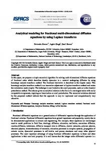
7 compact series), elliptic, eccentric, mean (least compact series). Indeed, for n < 0 expansion (3) in multiples of the true anomaly reduces to a nite polynomial. Moreover, the coecients Vsn;m (e) decrease faster than the coecients of expansions in multiples of other anomalies. On Figures 1{4 we see typical cases of the behavior of the coecients n;m n;m Vsn;m (e), Gn;m s (e), Ls (e), Ws (e) of expansions (3), (4), (6) and (9). Our calculations show that 1) the faster the series in multiples of a given anomaly converge, the larger is the maximal coecient of the corresponding series, and the smaller is the value of s for this maximal coecient; 2) the larger the value of m, the larger is the value of s for the maximal coecient of the corresponding expansion. For m=0 all four maximums correspond to s = 0 and the coecients decrease symmetrically with respect to s = 0 in accordance to the D'Alembert rule Xsn;m = X?n;s?m : (13) Let us note also an interesting phenomenon in the behavior of the Hansen coecients Ln;m s . For n + jmj = ?1 certain "pulsations" of the magnitude of the Hansen coecients can be observed (see, Figures 1{2). The "pulsations" appear only in the domain of increasing the Hansen coecients from the central minimum (Ln;m 0 (e) 0 for n + jmj = ?1). The number and the amplitude of the "pulsations" increases together with ?n. NUMERICAL COMPUTATION OF HANSEN-LIKE EXPANSIONS

2.5.2. Case n > 0 The expansions with n > 0 are used when considering, e.g., the perturbations due to external bodies. For n > 0 the anomalies can be ordered according to the compactness of the corresponding expansions as follows: eccentric, elliptic, true. In this case expansion (4) in multiples of the eccentric anomaly reduces to a nite polynomial. Numerical eciency of the expansions in multiples of the mean anomaly depends crucially on the precision to be acquired. For a low precision the series in multiples of the mean anomaly converge faster than the other ones. Because of a very fast decrease of the Hansen coecients these series are sometimes more ecient than even the series in multiples of the eccentric anomaly which have a nite number of terms (see, for example, Figure 5 in the neighborhood of maximum). For a higher precision the eciency of the series in multiples of the mean anomaly gets worse rapidly. n;m Figures 5{7 show typical behavior of Vsn;m (e), Gn;m s (e), Ls (e), n;m Ws (e) for n > 0. Our experiments show that the series in multiples of the mean anomaly are more ecient for larger values of n. The eciency of the series in multiples of the true anomaly decreases with increasing

8 SERGEI A. KLIONER ET AL. of n. The coecients Wsn;m(e) of the series in multiples of the elliptic anomaly do not decrease monotonically from the central maximum, but exhibit irregular pulsations of magnitudes (see, for example, Figure 5). Let us make some notes on the behavior of Hansen coecients. The larger the index m, the more asymmetric is the decrease of the Hansen coecients from the central maximum. This fact is observed visually on Figure 6. On the same Figure 6 we see that Hansen coecients exhibit again certain "pulsations" of magnitude. These "pulsations" are larger and more frequent for larger values of n and m. For larger eccentricities all the eects described above (e.g., number and amplitude of the "pulsations" for Hansen coecients, etc.) are ampli ed. Numerical eciency of all the expansions under consideration decreases with increasing the eccentricity. The described advantages and disadvantages of the anomalies for highly eccentric orbits are also ampli ed. On the opposite, for smaller eccentricities the dierences n;m n;m in the behavior of Vsn;m (e), Gn;m s (e), Ls (e), Ws (e) become smaller and the numerical eciency of all four kinds of expansions is almost the same. The results of our investigations are described in more detail in (Vasiliev, Vakhidov and Klioner, 1996). This work contains a large number of gures presenting the behavior of Fourier coecients for four representative values of the eccentricity: 0:1, 0:5, 0:75, 0:9. These gures con rm visually the eects described above. The gures, numerical values of the coecients as well as the software enabling one to compute the expansions are available from the authors upon request.

3. Derivatives of the Hansen-like Coecients Our approach allows one to evaluate not only the coecients Vsn;m (e), n;m n;m Gn;m s (e), Ls (e), Ws (e) but also their derivatives with respect to the eccentricity. It is very important because when constructing analytical and semi-analytical theories of motion we need to integrate dierential equations (for example, Lagrange equations or canonical equations for Delaunay variables) containing in the right-hand sides the derivatives of the perturbing function with respect to the orbital elements, rather than the perturbing function itself. We describe below how to solve this problem in the framework of our approach.

NUMERICAL COMPUTATION OF HANSEN-LIKE EXPANSIONS

9

3.1. True Anomaly We consider the left-hand side of (3) as a function of e and v

Fv (e; v) = 1 ? e

mv exp n 2

(1 + e cos v)n : Dierentiating this relation with respect to e we get @Fv = A F ; A = ?n 2e + cos v : v v v @e 1 ? e2 1 + e cos v On the other hand, we see that 1 dV n;m (e) @Fv = X s exp sv :

@e

s=?1

de

(14) (15) (16)

Therefore, the Fourier coecients of the function Av Fv coincide with the derivatives dVsn;m (e) =de we are looking for. In order to compute the Fourier expansion of Av Fv our approach described in Section 2 can be applied identically. The similar way can be used also for computing derivatives of the n;m n;m coecients Gn;m s (e), Ls (e) and Ws (e). 3.2. Eccentric Anomaly We consider the left-hand side of (4) as a function of e and g

Fg (e; g) = 1 ? e

mv ( e; g ) exp n 2

(1 + e cos v(e; g))n : Here v is considered as a function of e and g

g?e cos v = 1cos ? e cos g ; Using the equation @v (e; g) = sin v ; @e 1 ? e2 one gets

p

2 sin v = 11??eecossing g :

@Fg = A F ; A = 1 ?n (cos v + e) + m sin v : g g g 1 ? e2 @e

(17)

(18) (19) (20)

10 SERGEI A. KLIONER ET AL. 3.3. Mean Anomaly The left-hand side of (6) can considered as a function of e and l

Fl (e; l) = 1 ? e

mv ( e; l ) exp n 2

(21) (1 + e cos v(e; l))n ; where v is considered here as a function of e and l. Taking the derivative of (7) one gets @g (e; l) = psin v ; (22) @e 1 ? e2 @v (e; l) = sin v (2 + e cos v) : (23) @e 1 ? e2

and, therefore,

@Fl =A F ; @e l l Al = 1 ?1 e2 ?n cos v (1 + e cos v) + m sin v (2 + e cos v) :

(24)

3.4. Elliptic Anomaly The left-hand side of (9) can be considered as a function of e and w

Fw (e; w) = 1 ? e

mv ( e; w ) exp 2 n

(1 + e cos v(e; w))n : Here v is considered as a function of e and w. Hence we get

@Fw =A F ; @e w w @v (e; w) 2 v ? cos v en sin v Aw =n ?(12e+?e ecoscos + + m v) (1 ? e2 ) 1 + e cos v @e :

(25)

(26)

In order to compute @v (e; w) =@e we dierentiate one of the relations (18) taking into account that g is considered as a function of e and w here. The result is @v (e; w) = sin v + 1p+ e cos v @g (e; w) : (27) @e 1 ? e2 @e 1 ? e2 There are many ways to compute @g (e; w) =@e. We could, for example, dierentiate the series (11) with respect to e (the nome q depends only on the eccentricity e). Alternatively we could dierentiate in closed

11 form the de nition (10). Here we prefer another way, which avoids both expansions and the use of the elliptic amplitide am(x; e). Considering (8) as an implicit function for g(e; w) we get NUMERICAL COMPUTATION OF HANSEN-LIKE EXPANSIONS

@g (e; w) = ? @w (e; g) ?1 @w (e; g) ; @e @g " ? @e # @F g + 2 ; e K (e) ? F g + ; e dK (e) ; @w (e; g) = @e @e 2 de 2(K (e))2 ? @w (e; g) = @F g + 2 ; e ; (28) @g 2K (e) @g

and the derivatives of the elliptic integrals are de ned as

"

?

#

@F (; e) = 1 E (; e) ? 1 ? e2 F (; e) ? pe sin cos ; (29) @e 1 ? e2 e 1 ? e2 sin2 @F (; e) = p 1 ; (30) @ 1 ? e2?sin2 dK (e) = E (e) ? 1 ? e2 K (e) : (31) de (1 ? e2 ) e Here E (; e) and E (e) are the incomplete and complete elliptic integrals of the second kind, respectively. 3.5. Numerical Results In order to investigate the eciency of trigonometric series with the n;m n;m coecients dVsn;m (e) =de, dGn;m s (e) =de, dLs (e) =de, dWs (e) =de we have computed the series numerically for various eccentricities and for various values of n and m. We used herewith the software described in Section 3 generalized in an obvious way to cope with the functions (15), (20), (24) and (26). The results can be summarized as follows. For each anomaly the behavior of derivatives of the Fourier coecients is quite similar to the behavior of the Fourier coecients themselves as far as the eciency of the corresponding expansions is concerned. Numerical values of the derivatives are usually larger than the values of the coecients themselves. On Figures 8{10 one can see some examples of typical behavior of the derivatives. A large number of gures for the derivatives can be found in (Vasiliev et al., 1997). Additional gures, numerical values of the derivatives as well as the corresponding software are available from the authors upon request.

12 SERGEI A. KLIONER ET AL. 3.6. Higher-Order Derivatives n;m Computation of the higher-order derivatives of Vsn;m (e), Gn;m s (e), Ls (e), n;m Ws (e) (which are necessary for constructing of higher-order theories of motion) can be realized in essentially the same way as that of the rst-order derivatives. Indeed, let us consider the left-hand side of (1) as a function of e and an arbitrary anomaly x

Fx (e; x) = 1 ? e

mv ( e; x ) exp n 2

(32) (1 + e cos v(e; x))n ; where v is considered as a function of e and x. Using the approach described above we obtain quite generally

@Fx = A F : x x @e

(33)

@ 2 Fx = @Ax + (A )2 F : x x @e2 @e

(34)

1 d2 X n;m (e) @ 2 Fx = X s sx : exp @e2 s=?1 de2

(35)

One more dierentiation gives On the other hand,

Thus, the Fourier series of the right-hand side of (34) gives us the second-order derivatives d2 Xsn;m (e) =de2 . In the same way we could derive the \generating functions" for the derivatives of any order. Although for the higher-order derivatives the expressions are rather complicated, the derivation can be easily automated with the aid of any computer algebra system (what we in fact did even for the rst-order derivatives).

4. Concluding Remarks The approach described in the present paper enables one to evaluate by means of the fast Fourier transform not only the coecients considered in the paper and their derivatives, but also coecients of other Fourier expansions which are used in modern celestial mechanics. In the same way one can evaluate, for example, the Hansen-like coecients corresponding to other anomalies, the coecients of the generalized Kepler equation (see, Brumberg, 1992; Klioner, 1992), the functions F (e) and G (e) introduced in (Brumberg et al., 1995), Laplace coecients, etc. The derivatives of the corresponding coecients can be computed as

13 well. Simultaneous computation of a substantial numbers of harmonics allows one to judge how ecient the corresponding expansion is and how many terms are necessary to attain a required level of accuracy. In particular, our software enables one to calculate how many terms of an expansion we have to retain in order to represent the corresponding function of elliptic motion with a given accuracy. In principle, a similar FFT-based approach could be applied to investigate actual eciency of various variants of analytical and semi-analytical theories of motion of arti cial satellites and other celestial bodies (see, e.g., Klioner, 1997). A detailed study of the latter problem is underway. NUMERICAL COMPUTATION OF HANSEN-LIKE EXPANSIONS

Acknowledgements The authors are very grateful to Dr. Alexander M. Fominov for useful discussions. S.K. kindly acknowledges the receipt of a research fellowship of the Alexander von Humboldt Foundation.

References Bond V.R., Janin G.: 1981, Canonical orbital elements in terms of an arbitrary independent variable. Celest. Mech., 23, 159 Brumberg E.V.: 1992, Perturbed two-body motion with elliptic functions. Proc. 25th Symp. on Celest. Mech., NAO, Tokyo, 139 Brumberg E.V., Brumberg V.A., Konrad Th., Soel M.: 1995, Analytical linear perturbation theory for highly eccentric satellite orbits. Celest. Mech. and Dynam. Astron., 61, 369 Brumberg E.V., Fukushima T.: 1994, Expansions of elliptic motion based on elliptic function theory. Celest. Mech. and Dynam. Astron., 60, 69 Brumberg V.A., Klioner S.A.: 1995, Numerical eciency of the elliptic function expansions of the rst-order intermediary for general planetary theory. In: S.Ferraz-Mello, B.Morando, J.E.Arlot (eds.), Dynamics, ephemerides and astrometry in the solar system, Kluwer, Dordrecht, 101 Chapront J., Simon J.-L.: 1996, Planetary theories with the aid of the expansions of elliptic functions. Celest. Mech. and Dynam. Astron., 63, 171 Char B.W., Geddes K.O., Gonnet G.H., Leong B.L., Monagan M.B., Watt S.M.: 1993, MAPLE V Library Reference Manual. Springer, New York Danby J.M.A., Burkardt T.M.: 1983, The solution of Kepler's equation, I. Celest. Mech., 31, 95 Ferrandiz J.M., Ferrer S., Sein{Echaluce M.L.: 1987, Generalized elliptic anomalies. Celest. Mech., 40, 315 Goad C.C.: 1987, An ecient algorithm for the evaluation of inclination and eccentricity functions. Manuscripta Geodaetica, 12, 11 Klioner S.A.: 1992, Some typical algorithms of the perturbation theory within Mathematica and their analysis. Proc. 25th Symp. on Celest. Mech., NAO, Tokyo, 172 Klioner S.A.: 1997, On the Expansions of Intermediate Orbit for General Planetary Theory. Celest. Mech. and Dynam. Astron., in press Klioner S.A., Vakhidov A.A., Vasiliev N.N.: 1996, Fast Fourier transform for studying the convergence of elliptic motion series. Proc. of International Workshop "New computer technologies in control systems", Pereslavl-Zalessky, 34

14


Press W.H., Teukolsky S.A., Vetterling W.T., Flannery B.P., 1992. Numerical Recipes In Fortran: the art of scienti c computing. Cambridge University Press, New York Vakhidov A.A., Vasiliev N.N.: 1996, Development of analytical theory of motion for satellites with large eccentricities. Astron. Journ., 112, 2330 Vasiliev N.N., Vakhidov A.A., Klioner S.A.: 1996, On the convergence of elliptic motion series with dierent trigonometric arguments. ITA RAS Preprint, No 60 Vasiliev N.N., Vakhidov A.A., Klioner S.A.: 1997, Numerical computation of derivatives of Hansen{like coecients by means of the fast Fourier transform. ITA RAS Preprint, in press Vasiliev N.N., Vakhidov A.A., Sokolsky A.G.: 1996, Analytical theory of perturbations of the rst order in motion of a highly elliptic arti cial Earth satellite. ITA RAS Preprint, No 55

15

-200

Figure 1. The behavior of jVsn;mn;m (e)j (s 2 [?1; 39]), jGn;m s (e)j (s 2 [?48; 199]), n;m jLs (e)j (s 2 [?211; 895]), jWs (e)j (s 2 [?29; 142]) for e = 0:75, n = ?20, m = 19. Note that the series (3)n;m reduce to a polynomial for n < 0. Therefore, there exists only a nite number of Vs (e) in this case and all of them are shown on all Figures corresponding to n < 0. We intensionally show the behavior of the coecients for rather large values of jnj and jmj to make the behavior more clearly visible on the plots. To produce the coecients presented on all Figures of this paper we used 32 decimal digits arithmetic as implemented in Maple.

-18

-16

-14

-12

-10

-8

-6

-4

-2

0

2

4

6

8

10

log10|X n,m s |

V

0

W

G

200

s

400

600

L

800


16

-200 -20

-18

-16

-14

-12

-10

-8

-6

-4

-2

0

2

4

6

8

log10|X n,m s |

V

0

W

G

200

s

400

600

L

800


Figure 2. The behavior of jVsn;mn;m (e)j (s 2 [?1; 29]), jGn;m s (e)j (s 2 [?58; 175]), n;m jLs (e)j (s 2 [?275; 793]), jWs (e)j (s 2 [?34; 122]) for e = 0:75, n = ?15, m = 14.

17

-600 -20

-18

-16

-14

-12

-10

-8

-6

-4

-2

0

2

4

6

8

log10|X n,m s |

-400

-200

W

0 s

V

G

200

L

400

600


Figure 3. The behavior of jVsn;m (e)j (s 2 [?15; 15]), jGn;m s (e)j (s 2 [?123; 123]), n;m n;m jLs (e)j (s 2 [?600; 600]), jWs (e)j (s 2 [?80; 80]) for e = 0:75, n = ?15, m = 0.

18

-400

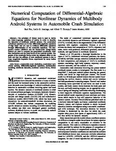
Figure 4. The behavior of jVsn;m (e)j (s 2 [?5; 15]), jGn;m s (e)j (s 2 [?90; 133]), n;m n;m jLs (e)j (s 2 [?456; 647]), jWs (e)j (s 2 [?56; 89]) for e = 0:75, n = ?10, m = 5.

-24

-22

-20

-18

-16

-14

-12

-10

-8

-6

-4

-2

0

2

4

log10|X n,m s |

-200

W

0

V

s

G

200

L

400

600


19

Figure 5. The behavior of jVsn;m (e)j (s 2 [?131; 131]), jGn;m s (e)j (s 2 [?20; 20]), n;m n;m jLs (e)j (s 2 [?145; 145]), jWs (e)j (s 2 [?64; 64]) for e = 0:75, n = 20, m = 0. Note that the series (4) reduce to a polynomial for n > 0. Therefore, there exists only a nite number of Gn;m s (e) in this case and all of them are shown on all Figures corresponding to n > 0.

-150

-24

-22

-20

-18

-16

-14

-12

-10

-8

-6

-4

-2

0

2

4

log10|X n,m s |

-100

W

-50

G

0 s

50

V

L

100

150


20

-100 n;m (e)j (s 2 [?111; 151]), jGn;m Figure 6. The behavior of jVsn;m s (e)j (s 2 [?20; 20]), n;m jLs (e)j (s 2 [?62; 360]), jWs (e)j (s 2 [?51; 73]) for e = 0:75, n = 20, m = 20.

-24

-22

-20

-18

-16

-14

-12

-10

-8

-6

-4

-2

0

2

4

log10|X n,m s |

G

0

W

100

s

V

200

L

300


21

Figure 7. The behavior of jVsn;m (e)j (s 2 [?106; 114]), jGn;m s (e)j (s 2 [?10; 10]), n;m n;m jLs (e)j (s 2 [?194; 297]), jWs (e)j (s 2 [?54; 59]) for e = 0:75, n = 10, m = 4.

-200

-26

-24

-22

-20

-18

-16

-14

-12

-10

-8

-6

-4

-2

0

2

log10|X n,m s |

-100

W

G

0

s

V

100

L

200

300


22

-200

Figure 8. The n;m behavior of jdVsn;m (e)=dej (s 2 n;m [?1; 39]), jdGn;m s (e)=dej (s 2 [?49; 202]), jdLs (e)=dej (s 2 [?219; 910]), jdWs (e)=dej (s 2 [?28; 140]) for e = 0:75, n = ?20, m = 19.

-16

-14

-12

-10

-8

-6

-4

-2

0

2

4

6

8

10

12

log10|dXn,m s /de| V

0

W

G

200

s

400

600

L

800


23

-600

Figure 9. The behavior of jdVsn;m (e)=dej (s 2 [?n;m 15; 15]), jdGn;m s (e)=dej (s 2 n;m [?124; 124]), jdLs (e)=dej (s 2 [?605; 605]), jdWs (e)=dej (s 2 [?81; 81]) for e = 0:75, n = ?15, m = 0.

-18

-16

-14

-12

-10

-8

-6

-4

-2

0

2

4

6

8

10

log10|dXn,m s /de|

-400

-200

W

0 s

V

G

200

L

400

600


24

-150

Figure 10. Then;mbehavior of jdVsn;m (e)=dej (s 2n;m [?136; 136]), jdGn;m s (e)=dej (s 2 [?20; 20]), jdLs (e)=dej (s 2 [?152; 152]), jdWs (e)=dej (s 2 [?66; 66]) for e = 0:75, n = 20, m = 0.

-24

-22

-20

-18

-16

-14

-12

-10

-8

-6

-4

-2

0

2

4

log10|dXn,m s /de|

-100

W

-50

G

0 s

50

V

L

100

150
