Numerical Simulations of Global-Scale High ...

JOURNAL OF GEOPHYSICAL RESEARCH, VOL. ???, XXXX, DOI:10.1029/,

Numerical Simulations of Global-Scale High-Resolution Hydrological Crustal Surface Deformations 1

1

R. Dill, H. Dobslaw,

R. Dill, Deutsches GeoForschungsZentrum GFZ, Section 1.3: Earth System Modelling, 14473 Potsdam, Germany, Tel.: +49-331-288 1750, Fax: +49-331-288 1163, ([email protected]) 1

Deutsches GeoForschungsZentrum GFZ,

Section 1.3: Earth System Modelling, 14473 Potsdam, Germany

D R A F T

October 15, 2014, 10:18am

D R A F T

X-2

DILL ET AL.: GLOBAL HIGH-RESOLUTION HYDRLOGICAL LOADING

Abstract.

High-resolution load-induced crustal surface deformations cal-

culated from numerical models are tested for their ability to predict hydrologically induced station height variations, as they reach comparable amplitudes as non-tidal atmospheric pressure loading known to be large enough to affect epoch-wise parameters obtained from the analysis of global geodetic networks. Loading contributions due to terrestrial water storage as given by global hydrological models are calculated on a 0.5◦ global regular grid with daily temporal resolution. Apart from the dominant seasonal variations, the hydrological loading signal discloses also rapid changes exceeding several millimeters that can be associated with major precipitation events and river floods. Locally strong loading signals with exceptionally high amplitudes, in many cases even with non-seasonal nature, occur along the major river channels. Only high-resolution loading calculations considering also the water mass anomalies stored in the model riverflow can resolve the correct amplitudes in the surrounded area up to 100 kilometers distance. The comparison of the modeled hydrological surface deformation with GPS station time series shows that high-resolution hydrological loading estimates based on global-scale models are able to explain large parts of the observed vertical station movements.

D R A F T

October 15, 2014, 10:18am

D R A F T

DILL ET AL.: GLOBAL HIGH-RESOLUTION HYDRLOGICAL LOADING

X-3

1. Introduction The Earth surface is deformed in response to temporal variations in the distribution of atmospheric, hydrological and oceanic mass loads imposed on the lithosphere. Besides tidal-induced mass variations, non-tidal mass variations with subdaily to seasonal periods lead to primarily vertical elastic deformations at global [Blewitt et al., 2001], regional [Fu et al., 2012] and local scales [Bevis, 2005]. In addition to atmospheric surface pressure, surface loading is mainly caused by hydrological mass re-distributions on seasonal time scales [e.g.

Tregoning et al., 2009; Rajner and Liwosz , 2011; Fritsche et al., 2012]. In

many places, the surface deformations are large enough to be detected with space geodetic techniques [Blewitt, 2003] and have to be taken into account for the realization of terrestrial reference frames as they can affect epoch-wise parameters causing a significant loss in solution accuracy [Dach and Dietrich, 2000]. Station-related load deformations can be calculated from sufficiently dense networks of station observations, or alternatively from global or regional numerical models. As mass variations induce deformation fields of principally global extent, generally, a large area around every station has to be taken into account. Mass variations from global hydrospheric models can provide the necessary basis for the calculation of large-scale deformation signals comparable to studies of deformation signals as detected by the satellite mission GRACE [van Dam et al., 2007, 2011] and additionally allow for the estimation of small-scale loading extremas, e.g. along river channels. Such location specific deformation signals can be found in many station height time series of GPS [Jiang et al., 2013; Williams and Penna, 2011; Rajner and Liwosz , 2011] and VLBI [Petrov and Boy, 2004] observations.

D R A F T

October 15, 2014, 10:18am

D R A F T

X-4

DILL ET AL.: GLOBAL HIGH-RESOLUTION HYDRLOGICAL LOADING

This study focuses on the calculation of high-resolution surface deformations using daily 0.5◦ global gridded terrestrial water storage variations of the global hydrological model LSDM [Land Surface Discharge Model; Dill , 2008]. Considering the extremely heterogeneous distribution of terrestrial water storage, e.g. across river channels, the load deformations are numerically integrated in the spatial domain based on Green’s function theory instead of the usual convolution approach in the spectral domain. Furthermore, we attempt to provide globally gridded deformation results suitable for extracting any local time series by interpolation. We present a patched Green’s function approach that is able to calculate high-resolution loading contributions on a sufficiently dense regular grid at daily time steps on standard computers. Although this approach is designed for all three deformation components, this paper concentrates on the prediction of the dominating vertical component. Local GPS solutions of station coordinates are compared to the hydrological loading contribution concerning the impact of river channel loads and sub-monthly variations and identifying prospects and limits for the modeling of station height variations by means of global hydrospheric models.

2. Global-Scale Gridded Surface Deformation Approach The crustal deformation of the Earth due to the gravitational and pressure induced stresses of surface mass loads can be expressed in the homogeneous and isotropic case by means of Load Love numbers depending on the spherical harmonic degree. In the spectral domain the set of Load Love numbers can be convolved with the global mass distribution to obtain global deformation fields. In the case of hydrological mass loads with sharply defined huge spatial mass differences the spectral convolution approach will lead to significant leakage errors because of using only a limited number of degrees and

D R A F T

October 15, 2014, 10:18am

D R A F T

DILL ET AL.: GLOBAL HIGH-RESOLUTION HYDRLOGICAL LOADING

X-5

orders. In the spatial domain the numerical computation of Earth surface deformations due to arbitrary load distributions is performed by using the fundamental Green’s function approach as described in Farrell [1972]. Load deformations at one specific point on the Earth surface are calculated as global sum of all point-mass contributions weighted by the distance depending Green’s functions. Farrell’s tabulated Green’s function, as used in this study, are based on the Load Love numbers for the Preliminary Reference Earth Model [PREM; Dziewonski et al., 1981]. Unlike tidal theory, surface loading theory includes a degree-one deformation generated by movement of the load center of mass with respect to the solid Earth center of mass. Therefore, the degree-one contributions entering the Green’s function summation depend on the choice of the reference frame and its moving origin. The Green’s function used here are specified in the center of mass of the solid Earth (CE) frame. For very accurate elastic load deformation according to Green’s function theory the summation of all global mass load contributions has to be done on a sufficiently dense spatial grid. As the computational costs for global spatial resolutions greater than 1.0◦ are generally to high for standard computing power, we attempt to separate the calculation of the globally gridded deformation field into a low-resolution far-field and a high-resolution near-field contribution exploiting the very smooth behavior of the Green’s function weights for large distance angles. The idea is to map the low-resolution far-field effect to a higher resolution by fast interpolation techniques and to substitute the high-resolution nearfield effect calculated only for a limited distance angle of a few degrees. To evaluate different choices for the far-field and near-field resolutions, the near-field distance angle and different interpolation techniques we set up a synthetic example.

D R A F T

October 15, 2014, 10:18am

D R A F T

X-6

DILL ET AL.: GLOBAL HIGH-RESOLUTION HYDRLOGICAL LOADING

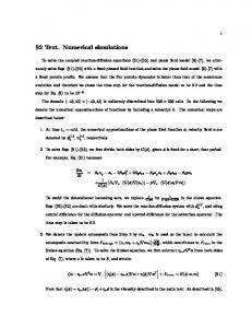
3. Required Spatial Resolution: A Synthetic Example The synthetic example gives the spatial loading calculation for a typical hydrological surface mass distribution in the area of a large river channel. Fig. 1 shows a cross-section of the simulated mass load and deformation representing the loading effect due to the water storage around Manaus City, located at the Rio Negro and the Amazon river, during stage height maximum in June. The 2D-test mass (red line on top) is discretized on a model-like 0.5◦ regular grid (green dots). Additionally, a spatially filtered (Gauss, R = 500 km) mass representation on a 1.0◦ grid, approximating a GRACE satellite observation, is given (grey dots). The high-resolution near-field calculation is done with a gridded mass distributions resampled to 0.01◦ . Based on Green’s function theory, vertical load deformations are calculated from these three mass distributions by summation of all loads according to the distance-weights given by the Greens functions. The red line (bottom) gives the expected elastic surface deformation with 38.9 mm in the maximum centered at the river channels containing 4.0 m river mass load. At Manaus station, 10 km away from the riverside, one would observe a depression of 28.1 mm. From the two gridded mass distributions, and its resampled high-resolution versions the vertical load deformations along the cross-section are calculated on three different sample intervals: at station locations every 0.01◦ , gridded every 0.5◦ , and every 1.0◦ . Using the 0.5◦ gridded mass distributions, the brown dots give the deformations at every 1.0◦ grid point and the green dots at every 0.5◦ grid point. The dotted lines, connecting the colored dots represent a cubic spline interpolation within the gridded deformation results to extract the load deformations at intermediate locations. In principle, we expect most accurate loading results when calculating the deformation directly at each station location

D R A F T

October 15, 2014, 10:18am

D R A F T

DILL ET AL.: GLOBAL HIGH-RESOLUTION HYDRLOGICAL LOADING

X-7

as it is shown by the solid colored lines. As the loading Green’s function weight changes rapidly for distance angles below 0.5 − 1.0◦ the broadening of the sharp mass maximum in the river channels over one whole 0.5◦ model-gridcell reduces significantly the deformation amplitude. At Manaus station we would obtain only 22.9 mm, about 81.5% of the true deformation. To consider the enhanced Green’s function weights for low distances, we have to switch to a high-resolution near-field calculation based on the resampled version of the gridded mass distribution. The blue dots show the deformation according to this resampled mass distribution, calculated again every 0.5◦ , and the solid blue line shows the related station-wise (every 0.01◦ ) result. The deformation amplitude at our test location in Manaus increases to 24.1 mm (95.1%). A cubic spline interpolation between the 0.5◦ gridded deformation points yield almost the same result by reducing the computational effort significantly at the same time. Starting with a mass distribution that is discretized on only 1.0◦ we obtain a maximum deformation signal similar to the brown dotted line, recovering not more than 68% of the loading signal at Manaus station. All simulation results based on gridded mass distributions suffer from the fact, that the deformation maximum appears always below the gridcell centers of the model mass distribution. The coarser the model mass is discretized, the more the real localization of the depression maximum gets lost. Depending on the location of the real load maximum inside the model mass grid, the high-resolution near-field approach can even enhance this feature leading potentially to deformation amplitudes even overestimated by 17%. For distances from the river channels greater than one gridcell size the deviations due to this maximumshift keep below 2.5%, whatever approach is applied. The GRACE like filtered mass distribution cannot resolve such narrow mass loads from rivers at all, leading to only

D R A F T

October 15, 2014, 10:18am

D R A F T

X-8

DILL ET AL.: GLOBAL HIGH-RESOLUTION HYDRLOGICAL LOADING

a third of the deformation amplitude (grey dots and line). Further calculations using much lower resolutions, only 2.0◦ for mass and 2.5◦ for stations, and analogous analysis of the horizontal deformation components, not shown in the figure, lead to our final patching approach for the calculation of global load deformations: The deformation is calculated every 2.5◦ on a regular global grid using a 2◦ model mass distribution. This 2.5◦ deformation field is interpolated to 0.5◦ . The near-field loading contribution inside a 6◦ × 6◦ box around every station (≈ ±3◦ distance) is replaced by a high-resolution calculation carried out every 0.5◦ on a regular global grid using a 0.125◦ model mass distribution. This procedure is more than 1000 times faster than the full spatial integration for stations every 0.5◦ using a 0.125◦ mass distribution and even three times faster than the comparable spectral approach up to degree and order 1440. Deviations between the three approaches keep below 1.8%.

4. Non-tidal Load Deformation From Hydrology, Atmosphere, Ocean For this study we analyze two years of global hydrological surface deformation fields calculated every 0.5◦ at daily time steps according to water storage estimates for the years 2010 and 2011 from LSDM [Land Surface Discharge Model; Dill , 2008]. LSDM continental water storage considers snow accumulation, seasonal runoff from glaciers, and water flow in river channels given as daily states on a 0.5◦ regular global grid. Additionally, we processed consistent deformation fields for the ECMWF (European Centre for MediumRange Weather Forecasts) atmospheric surface pressure and the OMCT [Ocean Model for Circulation and Tides; Dobslaw and Thomas, 2007] non-tidal ocean bottom pressure to derive the total non-tidal deformation signal. For comparison, we take also two years of corresponding global deformation estimates from the Global Geophysical Fluids Center

D R A F T

October 15, 2014, 10:18am

D R A F T

DILL ET AL.: GLOBAL HIGH-RESOLUTION HYDRLOGICAL LOADING

X-9

(GGFC) of the International Earth Rotation and Reference Systems Service (IERS). The GGFC provides precomputed daily surface deformation fields with 2.5◦ × 2.5◦ spacing of non-tidal ocean loading1 based on ocean bottom pressure fields from the Estimating the Circulation and Climate of the Ocean (ECCO) project and non-tidal atmospheric loading2 based on surface pressure field variations provided by the National Centers for Environmental Prediction (NCEP). GGFC links also to a provisional hydrological loading product3 with monthly time series at 170 stations and globally gridded 1.0◦ × 1.0◦ load displacements (last month of data released was 09/2011) using data from the GLDAS NOAH hydrology model [Rodell et al., 2004]. One has to be aware that the loading product based on GLDAS accounts only for soil moisture, snow water equivalent and canopy water, whereas riverflow is not included. Ice sheet processes and areas with permafrost were also masked out for the GLDAS load calculations. Deep groundwater variations are not modeled by GLDAS nor in the LSDM model. For all load calculations a landsea mask at 0.25◦ grid size was applied to improve the representation of the coastal discontinuities due to continental water storage anomalies limited to land areas and the fundamentally different response of the solid Earth and the oceans to surface pressure variations. For the remainder of this study we label the gridded deformation results according to their underlying model masses as LSDM-, GLDAS-, ECMWF-, NCEP-, OMCT-, ECCO-loading. Figure 2a gives the RMS amplitudes of the LSDM-loading deformation. Vertical displacements due to terrestrial water storage can regionally exceed the atmospheric loading signal, with highest amplitudes, up to ±30 mm modeled in the Amazon basin. The hydrological signal has generally a dominant seasonal character and at least 80% of the total

D R A F T

October 15, 2014, 10:18am

D R A F T

X - 10

DILL ET AL.: GLOBAL HIGH-RESOLUTION HYDRLOGICAL LOADING

deformation variance can be explained by monthly mean variations. Nevertheless, also after removing monthly means from the daily LSDM-loading signal, there remain submonthly variations with RMS amplitudes exceeding still several millimeters (Fig. 2b). The largest non-seasonal contributions are located in regions with also high seasonal amplitudes and, additionally, along the courses of the major rivers like Amazon, Nile, and Lena. Major medium-scale patterns in hydrological induced continental crustal deformation are comparably predictable by both, LSDM and GLDAS. On the seasonal time scale, largest differences in amplitude between both loading predictions occur along the Rocky Mountains, the Amazon basin, Rio de la Plata basin, and the Himalayan Plateau. Figure 3a gives a global overview on the agreement between LSDM-loading and GLDAS-loading. Green areas indicate an agreement in amplitude (1.0 ± 0.25) given as standard deviation of LSDM in relation to GLDAS and also high correlations (> 0.7). Low correlations can be found in North Africa where the signal amplitudes are generally tiny, and along major rivers like Nile, Lena, Ob, and Yenisei, where only LSDM-based loading results capture the local effect of the river mass loads along the river side. In the Amazon region and along the north-west coast of North America, LSDM derived deformations correlate very well with GLDAS results, but LSDM predicts much higher amplitudes, which might be related to different forcing data but also to the lower temporal and spatial resolution of the GLDAS data employed. Small-scale features like river storage, filling of dams and lakes, not considered in the GLDAS water masses, lead to a further underestimation of a few millimeters, along the Amazon river channel even up to 16 mm. One should also keep in mind that frozen regions, like Greenland are mask out in the GLDAS calculations. Fitting an annual signal to both data sets, we note largely comparable phases, except in the

D R A F T

October 15, 2014, 10:18am

D R A F T

DILL ET AL.: GLOBAL HIGH-RESOLUTION HYDRLOGICAL LOADING

X - 11

region of Siberia and Alaska, where the model parametrizations might cause differences in the melting on-set and melting speed of the snow pack. Whereas the annual phase estimates from LSDM agree well with GRACE estimates [end of June to mid of July, see Eriksson and Macmillan, 2012], the GLDAS data set indicates a slightly later maximum in the loading amplitude. Comparing the hydrological loading contribution to the deformation signal from atmospheric surface pressure and ocean bottom pressure, atmospheric loading dominates the total loading signal over most part of the northern hemisphere. In the Rocky Mountains and in Western Europe hydrological loading reaches 50% of the total signal. Load deformations in arid region are exclusively caused by atmospheric pressure loading but their amplitudes are two to five times lower, only 1 - 2 mm. The tropics, especially the Amazon basin, the Eastern part of the Rocky Mountains and the Himalayan region, North Australia and additionally locations at lake- and riversides are dominated by hydrological loading. Figure 3b compares the total model based surface load displacement for two model combinations. The agreement in total vertical deformation between ECMWF+OMCT+LSDM and NCEP+ECCO+GLDAS benefits from the good agreement of ECMWF-loading and NCEP-loading. Their correlation in time is generally above 0.8 with only two exception in Central Asia and Eastern Africa showing correlation of only 0.6. In contrast to hydrologic and atmospheric loading, non-tidal ocean loading causes significant contributions only in a few coastal regions around shallow water ocean basins and along the Antarctic coastline, generally below 2 mm. Most of the differences in amplitude (standard deviation) between both model combinations can be attributed to differences in the loading results from LSDM and GLDAS.

D R A F T

October 15, 2014, 10:18am

D R A F T

X - 12

DILL ET AL.: GLOBAL HIGH-RESOLUTION HYDRLOGICAL LOADING

5. Comparison With GPS Height Variation To apply simulated crustal deformations to space-geodetic observations, we select 53 globally distributed GPS station sites, where appropriate station coordinate time series were easily available from the data service centers of the International GNSS service (IGS4 ), the Geocentric Reference System for the Americas (SIRGAS5 ), the US universitygoverned facility center UNAVCO6 or the European permanent GNNS network EUREF7 . GPS station time series are taken from the weekly solutions as they are published from the service centers. The time series of predicted station deformations from the models are extracted from the global gridded deformation fields at the station location by bicubic spline interpolation avoiding interpolation across the coastline. Note, that for the following comparison we do not transform the ellipsoidal heights from the GPS solutions into geocentric vertical directions as given by the deformation models, since we believe the small differences are negligible here. The correlation between the predicted total vertical displacement from ECMWF+OMCT+LSDM and the GPS observed station height variation generally exceeds 0.6 for the selected inland stations, whereas GPS height series at coastal stations show much higher variability and higher amplitudes than the predictions from OMCT and ECCO. Far from the coast only at Alchevsk (ALCI) and Zimmerwald (ZIMM) the correlations are low. Though the predicted vertical displacement varies with an comparable amplitude they are not in phase with the GPS results. In case of Alchevsk the loading signal is dominated by hydrology, simulated with a maxima in March by LSDM, and likewise by GLDAS, but GPS observes a maxima in May. In Zimmerwald hydrological loading adds a seasonal signal to

D R A F T

October 15, 2014, 10:18am

D R A F T

X - 13

DILL ET AL.: GLOBAL HIGH-RESOLUTION HYDRLOGICAL LOADING

the high-frequency atmospheric loading, both of the same magnitude and the maxima of hydrological loading follows the observed maxima in January by about 1-2 months. The following figures 5 - 11 exemplify some typical hydrological loading contributions at specific continental station locations. For better visual comparison of the weekly GPS time series with the total modeled deformation (ECMWF+OMCT+LSDM and NCEP+ECCO+GLDAS), a box-car filter of 28 days is applied to these three time series. Station Smila (SMLA, Fig. 5) in Ukraine and station Budapest (BUTE, Fig. 6) represent typical continental sites with large surface deformations caused by atmospheric surface pressure and a seasonal contribution of about the same order of magnitude from hydrological loading. The totally predicted deformation coincides very well with the GPS solution in both, amplitude and phase, leading to correlation of 0.79. At Budapest the daily LSDM model predicts additional sub-seasonal variability after the melting season in June and July of about 2 mm, presumably caused by local Danube river loads. These non-seasonal features could be hardly assigned to related variations in the observed GPS time series because the weekly GPS solution is dominated by higher-frequency variations of atmospheric loading. At Norilsk (NRIL, Fig. 7) in Siberia the hydrological mass loads are mainly determined by snow coverage and snow melting processes. The resulting loading signals in LSDM and GLDAS show both a typical seasonal saw tooth variation of about the same amplitude but with slightly different phases. As the total deformation signal is highly affected by the short period atmospheric surface pressure loading, the correct phase could not be determined from those short GPS time series. Analysis of longer time series may provide

D R A F T

October 15, 2014, 10:18am

D R A F T

X - 14

DILL ET AL.: GLOBAL HIGH-RESOLUTION HYDRLOGICAL LOADING

the necessary information about the correct phase, helping to improve the melting process parametrization of global hydrological models. In the Amazon basin we find the largest hydrological surface deformations due to extremely high water storage variations and additional high river channel loads. The station site displacements at Manaus (NAUS, Fig. 8) and Porto Velho (POVE, Fig. 9) are prominently dominated by the annual rainfall season. In Manaus GPS observes 50 - 75 mm, in Porto Velho 30 - 40 mm peak-to-peak amplitude in the up component. In contrast to Porto Velho, the Manaus station is located directly at the riverbank of Rio Negro only a few kilometers upstream from the Amazon river and the loading signal is heavily influenced by variable water loads inside the river channel. At Manaus LSDM predicts a maximum vertical surface deformation with around 80% of the observed up component measured by GPS, which is well in line with the theoretically expected value of 95% that could be obtained from a 0.5◦ regular gridded mass distribution as discussed before in section 3 (Fig. 1). The slightly lower loading signal may be attributed to deficiencies in the modeled station-to-river distance due to the approximated location of the model river path in the river routing scheme. LSDM-loading obtains a correlation of 0.91 with the GPS time series having a predicted phase of the annual amplitude that trails the GPS observed by about 14 days. GLDAS-loading cannot recover the observed amplitude, presumably due to the unconsidered water masses in the river channel and a coarser resolution of the provided deformation field. Like in LSDM the correlation is also high with 0.73; it is having a phase lag of -28 days. At Porto Velho, representing more or less only the large-scale deformation in the Amazon basin far away from the Amazon main river channel, LSDM and GLDAS correlate with the GPS station height variation by about

D R A F T

October 15, 2014, 10:18am

D R A F T

DILL ET AL.: GLOBAL HIGH-RESOLUTION HYDRLOGICAL LOADING

X - 15

0.80, both with a phase lag of -21 days. This is a fairly excellent result for global-scale model predictions attesting almost correctly simulated water mass storage and transport processes in the Amazon basin by both hydrological models. Like the Manaus station, the GPS station in Wuhan (WUHN, Fig. 10) in China is located only 6 km away from the Yangtze River surrounded by many lakes. GPS observes up to 20 mm peak-to-peak vertical amplitudes with a maxima in August and a minima in February corresponding to the annual variation in river discharge between wet and dry season. LSDM can explain the major parts of the station up component, for 2010 almost perfectly in amplitude and phase. Again, GLDAS underestimates the loading signal due to the neglected river channel masses. Sub-monthly variations with amplitudes of 10 mm can be attributed to variations in atmospheric surface pressure that cancel out partly the seasonal hydrological loading signal. The last example shows a GPS station in Darwin (DARW, Fig. 11) in northern Australia situated in the upstream part of the Darwin Harbour catchment close to the Manton reservoir. Water storage in that region depends primarily on the precipitation intensity during the short wet season from December to March and the dry season from June to October. Additionally, water storage variations are highly affected by human water regulations not considered in the models LSDM and GLDAS. The Manton dam serves as water reservoir for the Northern Territories citys, but since the construction of the Darwin River Dam in 1972, the water storage at Manton Dam serves only as back-up supply for Darwin, and is used for recreation. In the model predictions we find a typical seasonal hydrological loading contribution of 10-15 mm vertical deformation superimposed by a mainly seasonal atmospheric signal of 5 mm with about 3-4 month phase difference. The

D R A F T

October 15, 2014, 10:18am

D R A F T

X - 16

DILL ET AL.: GLOBAL HIGH-RESOLUTION HYDRLOGICAL LOADING

GPS solution shows much more intra-seasonal variations due to human water regularization and withdraw in the network of reservoirs around Darwin that are not predictable by the models. In case of GLDAS the hydrological loading amplitude seems to be much too low, whereas in LSDM water storage variations are presumably overestimated by too large precipitation rates and a too late onset of the rainy season in the ECMWF forcing data.

6. Conclusions High-resolution global-scale surface deformations calculated daily at 0.5◦ global grids from modeled mass distributions of global hydrospheric model outputs for atmosphere, ocean, and continental hydrology are analyzed and compared to GPS station height variations in terms of its high-resolution spatial and temporal signal content. Special focus of this study is on the influence of different spatial and temporal resolutions of the global model outputs and the global deformation calculation concerning especially hydrological water loads. Water mass loads are taken from daily simulated LSDM water storage data, that include not only soil moisture and snow accumulation but also the water stored in river channels and lakes. The hydrological loading signal exceeds the atmospheric loading contribution in many regions. In comparison to the low-resolution loading product based on GLDAS (1.0◦ , monthly, no surface water) the LSDM (0.5◦ , daily, incl. surface water) based high-resolution loading calculation is able to resolve much higher amplitudes prominently along the major river paths of Lena, Ob, Nile, and Amazon. In addition to a significant phase shift against the surrounding region, this river loading contributions contain also sub-monthly variations of several millimeters in the vertical deformation. The comparison of the modeled loading results with GPS station coordinates indicates that

D R A F T

October 15, 2014, 10:18am

D R A F T

X - 17

DILL ET AL.: GLOBAL HIGH-RESOLUTION HYDRLOGICAL LOADING

they are highly affected by seasonal hydrological deformations. To exploit the full potential of modeled global water variations, typically given as daily values on a 0.5◦ regular grid it is mandatory to calculate the deformation fields on the same temporal resolution with at least 0.5◦ spatial resolution and to consider the water masses stored in the model riverflow component. It turns out that for stations located near riverbanks, the approximated locations of the model river channels, defined from the 0.5◦ river routing scheme, are not sufficient. The deviation of the model river location from their real geographic river channel positions can reach up to 50 km leading to vertical loading errors of up to 28%. The horizontal deformation components are even much more affected by this localization problem of the model river paths. The challenge will be to locate the riverflow masses stored in the model more precisely to the high-resolution 0.125◦ resampled mass distribution used for the loading calculation. This study prefers the calculation of global-scale deformation maps as they offer the opportunity to categorize regions according to their individual influences of nontidal atmospheric, oceanic, and hydrological loading contributions. Additionally to local station height corrections, global loading patterns can support decisions concerning geodetic network station distributions and help to interpret comparisons of epochwise parameters obtained from the analysis of differently distributed global geodetic networks. Both current global hydrospheric model combinations (ECMWF+OMCT+LSDM and NCEP+ECCO+GLDAS) are able to predict more than 60% of the observed GPS height variations at almost all of the considered continental stations sites.

Since

ECMWF+OMCT+LSDM are principally available in real time, modeled surface deformations are now in aposition to be introduced into geodetic network analysis. Furthermore,

D R A F T

October 15, 2014, 10:18am

D R A F T

X - 18

DILL ET AL.: GLOBAL HIGH-RESOLUTION HYDRLOGICAL LOADING

the comparison of geodetic station coordinates and hydrological surface deformations offer a new possibility to improve hydrological model processes like water mass residence and transport parametrization (e.g by irrigation or dams), discharge velocities, or snow melting processes. In return, the comparison of the GPS observation with the separated contributions of non-tidal local surface deformations opens up a wide area for the interpretation of GPS derived surface movements. Acknowledgments. Deutscher Wetterdienst, Offenbach, Germany, and the European Centre for Medium-Range Weather Forecasts are acknowledged for providing data from ECMWF’s operational model. Numerical simulations were performed at Deutsches Klimarechenzentrum DKRZ, Hamburg, Germany.

Notes 1. van Dam, T., 2010, http://geophy.uni.lu/ggfc-oceans.html

2. van Dam, T., 2010, http://geophy.uni.lu/ncep-loading.html

3. from the NASA GSFC VLBI group, http://lacerta.gsfc.nasa.gov/hydlo (Eriksson & MacMillan)

4. ftp.//cddis.gsfc.nasa.gov/pub/gps/products

5. ftp://ftp.sirgas.org/pub/gps/SIRGAS

6. ftp.//data-out.unavco.org/pub/products/position

7. ftp.//igs.bkg.bund.de/EUREF/products

References Bevis, M. (2005), Seasonal fluctuations in the mass of the Amazon River system and Earths elastic response. Geophysical Research Letters, 32, 36, :10.1029/2005GL023491.

D R A F T

October 15, 2014, 10:18am

D R A F T

X - 19

DILL ET AL.: GLOBAL HIGH-RESOLUTION HYDRLOGICAL LOADING

Blewitt, G., Lavallee, D., Clarke, P. and K. Nurutdinov (2001), A new global mode of Earth deformation: Seasonal cycle detected, Science, 294, 23422345. Blewitt, G. (2003), Self-consistency in reference frames, geocenter definition, and surface loading of the solid Earth, Journal of Geophysical Research, 10.1029/2002JB002082. Dach, R., and R. Dietrich (2000), Influence of the ocean loading effect on GPS derived precipitable water vapor, Geophysical Research Letters, 2000, 27, 29532956. Dill, R. (2008), Hydological model LSDM for operational Earth rotation and gravity field variations, Scientific Technical Report, STR08/09, GFZ Potsdam, Germany, 35p. Dobslaw, H. and M. Thomas (2007), Simulation and observation of global ocean mass anomalies Journal of Geophysical Research, 112, 10.1029/2006JC004035. Dziewonski, A. M., and D. L. Anderson (1981), Preliminary Reference Earth Model, Phys. Earth Planet. Inter., 25, 297356. Eriksson,

D.

Loading

and

Observed

D.S. by

Macmillan VLBI

(2012),

Continental

Measurements,

Poster

Hydrology presentation:

http://www.oan.es/gm2012/pdf/poster id 84.pdf. Farrell, W.E. (1972), Deformation of the Earth by surface loads, Reviews of Geophysics, 10, 751-797. Fritsche, M., D¨oll, P. and R. Dietrich (2012), Global-scale validation of model-based load deformation of the Earths crust from continental watermass and atmospheric pressure variations using GPS, Journal of Geodynamics, 59-60, 133142. Fu, Y., Freymueller, J.T. and T. Jensen (2012), Seasonal hydrological loading in southern Alaska observed by GPS and GRACE, Geophysical Research Letters, 39, L15310.

D R A F T

October 15, 2014, 10:18am

D R A F T

X - 20

DILL ET AL.: GLOBAL HIGH-RESOLUTION HYDRLOGICAL LOADING

Jiang, W., Li, Z., van Dam, T. and W. Ding (2013), Comparative analysis of different environmental loading methods and their impacts on the GPS height time series, Journal of Geodesy, 87, 687-703, 10.1007/s00190-013-0642-3. Petrov, L., and J.-P. Boy (2004), Study of the atmospheric pressure loading signal in VLBI observations, Journal of Geophysical Research, 109, 114. Rajner, M. and T. Liwosz (2011), Studies of crustal deformation due to hydrological loading on GPS height estimates, Geodesy and Cartography, 60, 135144, 10.2478/v10277012-0012-y. Rodell, M., Houser, P.R., Jambor, U. et al. (2004), The Global Land Data Assimilation System, Bulletin of the American Meteorological Society, 85, 381394, 10.1175/BAMS85-3-381. Tregoning, P., Watson, C. and G. Ramillien (2009), Detecting hydrologic deformation using GRACE and GPS, Geophysical Research Letters, 36, L15401. van Dam, T., Collieux, X., Altamimi, Z. and J. Ray (2011), A review of GPS and GRACE estimates of surface mass loading effects, In: Presentation EGU Vienna 2011. van Dam, T., Wahr, J. and D. Lavalle (2007), A comparison of annual vertical crustal displacements from GPS and Gravity Recovery and Climate Experiment (GRACE) over Europe, Journal of Geophysical Research, 112, 111, 10.1029/2006JB004335. Williams, S.D.P. and N.T. Penna (2011), Non-tidal ocean loading effects on geodetic GPS heights, Geophysical Research Letters, 38, L09314.

D R A F T

October 15, 2014, 10:18am

D R A F T

DILL ET AL.: GLOBAL HIGH-RESOLUTION HYDRLOGICAL LOADING

X - 21

figures/loadinterpolation_reduced_only0.5.eps

Figure 1.

Surface deformations from a synthetic river load in the Amazon basin. Top:

Cross-section of simulated 2D-mass distribution as equivalent water height [cm] (red line) and its representation on a 0.5◦ grid (green dots), and spatially smoothed (R = 8◦ ≈ 400km) on a 1.0◦ grid (grey dots). Bottom: Calculated vertical deformation profiles around Manaus, ±3◦ distance. Red line is the expected deformation profile according to the mass load. For three different mass distributions (0.5◦ and 0.5◦ resampled to 0.01◦ , and 1.0◦ spatially smoothed) the deformation is calculated continuously (at station locations, solid lines) and as 0.5◦ and 1.0◦ gridded deformation field (colored dots). Dotted lines represent cubic spline interpolation within the gridded deformation fields.

D R A F T

October 15, 2014, 10:18am

D R A F T

X - 22

DILL ET AL.: GLOBAL HIGH-RESOLUTION HYDRLOGICAL LOADING

figures/deformv_LSDM_2011_RMS_both.eps

Figure 2. RMS amplitudes of continental hydrological loading from daily LSDM water storage 2010 - 2011 [mm]. a) total vertical deformation, b) non-seasonal part (monthly means removed).

figures/STD_CORR_both.eps

Figure 3.

Agreement of hydrological loading from a) LSDM and GLDAS,

b) ECMWF+OMCT+LSDM and NCEP+ECCO+GLDAS. Agreement in standard deviation is coded in colors from blue (LSDMGLDAS). Correlation lower than 1.0 are coded as color modulation damping the saturation. Green areas indicate high correlation and equal amplitudes of both models.

D R A F T

October 15, 2014, 10:18am

D R A F T

X - 23

DILL ET AL.: GLOBAL HIGH-RESOLUTION HYDRLOGICAL LOADING

figures/CORR_ECMWFOMCTLSDM_GPS_s.eps

Figure 4. Correlation between modeled vertical displacement from ECMWF+OMCT+LSDM and up-coordinate at 53 GPS stations.

figures/SMILA_deformv_ssc.eps

Figure

5.

Vertical displacement at GPS station Smila in Central Eu-

rope.

Modeled contribution due to ATML (cyan=NCEP, blue=ECMWF), NTOL

(magenta=ECCO, and

filtered

(28

red=OMCT), day

boxcar)

and total

HYDL sum

(dark

green=GLDAS,

green=LSDM)

(orange=NCEP+ECCO+GLDAS,

dark

red=ECMWF+OMCT+LSDM). GPS station heights are given as original weekly solutions (black dots=IGS/EUREF/SIRGAS) and as monthly fit (black line). Correlation between GPS and models are ECMWF+OMCT+LSDM=0.70, ECMWF+OMCT+LSDM filtered=0.79, NCEP+ECCO+GLDAS=0.80, NCEP+ECCO+GLDAS filtered=0.89.

D R A F T

October 15, 2014, 10:18am

D R A F T

X - 24

DILL ET AL.: GLOBAL HIGH-RESOLUTION HYDRLOGICAL LOADING

figures/BUDAPEST_deformv_ssc.eps

Figure

6.

Vertical displacement at GPS station Budapest in Central Eu-

rope.

Modeled contribution due to ATML (cyan=NCEP, blue=ECMWF), NTOL

(magenta=ECCO, and

filtered

(28

red=OMCT), day

boxcar)

and total

HYDL sum

(dark

green=GLDAS,

green=LSDM)

(orange=NCEP+ECCO+GLDAS,

dark

red=ECMWF+OMCT+LSDM). GPS station heights are given as original weekly solutions (black dots=IGS/EUREF/SIRGAS) and as monthly fit (black line). Correlation between GPS and model are ECMWF+OMCT+LSDM=0.70, ECMWF+OMCT+LSDM filtered=0.79, NCEP+ECCO+GLDAS=0.69, NCEP+ECCO+GLDAS filtered=0.73.

D R A F T

October 15, 2014, 10:18am

D R A F T

X - 25

DILL ET AL.: GLOBAL HIGH-RESOLUTION HYDRLOGICAL LOADING

figures/NORILSK_deformv_ssc.eps

Figure 7.

Vertical displacement at GPS station Norilsk in Siberia.

Mod-

eled

due

(ma-

contribution

genta=ECCO, and

filtered

to

red=OMCT), (28

day

ATML and

boxcar)

(cyan=NCEP, HYDL

total

sum

(dark

blue=ECMWF),

NTOL

green=GLDAS,

green=LSDM)

(orange=NCEP+ECCO+GLDAS,

dark

red=ECMWF+OMCT+LSDM). GPS station heights are given as original weekly solutions (black dots=IGS/EUREF/SIRGAS) and as monthly fit (black line). Correlation between GPS and models are ECMWF+OMCT+LSDM=0.52, ECMWF+OMCT+LSDM filtered=0.55, NCEP+ECCO+GLDAS=0.47, NCEP+ECCO+GLDAS filtered=0.40.

D R A F T

October 15, 2014, 10:18am

D R A F T

X - 26

DILL ET AL.: GLOBAL HIGH-RESOLUTION HYDRLOGICAL LOADING

figures/MANAUS_deformv_ssc.eps

Figure

8.

Vertical displacement at GPS station Manaus at the Ama-

zon.

Modeled contribution due to ATML (cyan=NCEP, blue=ECMWF), NTOL

(magenta=ECCO, and

filtered

(28

red=OMCT), day

boxcar)

and total

HYDL sum

(dark

green=GLDAS,

green=LSDM)

(orange=NCEP+ECCO+GLDAS,

dark

red=ECMWF+OMCT+LSDM). GPS station heights are given as original weekly solutions (black dots=IGS/EUREF/SIRGAS) and as monthly fit (black line). Correlation between GPS and models are ECMWF+OMCT+LSDM=0.91, ECMWF+OMCT+LSDM filtered=0.92, NCEP+ECCO+GLDAS=0.73, NCEP+ECCO+GLDAS filtered=0.74.

D R A F T

October 15, 2014, 10:18am

D R A F T

X - 27

DILL ET AL.: GLOBAL HIGH-RESOLUTION HYDRLOGICAL LOADING

figures/PORTOVELHO_deformv_ssc.eps

Figure 9. zon.

Vertical displacement at GPS station Porto Velho at the Ama-

Modeled contribution due to ATML (cyan=NCEP, blue=ECMWF), NTOL

(magenta=ECCO, and

filtered

(28

red=OMCT), day

boxcar)

and total

HYDL sum

(dark

green=GLDAS,

green=LSDM)

(orange=NCEP+ECCO+GLDAS,

dark

red=ECMWF+OMCT+LSDM). GPS station heights are given as original weekly solutions (black dots=IGS/EUREF/SIRGAS) and as monthly fit (black line). Correlation between GPS and models are ECMWF+OMCT+LSDM=0.73, ECMWF+OMCT+LSDM filtered=0.84, NCEP+ECCO+GLDAS=0.80, NCEP+ECCO+GLDAS filtered=0.82.

D R A F T

October 15, 2014, 10:18am

D R A F T

X - 28

DILL ET AL.: GLOBAL HIGH-RESOLUTION HYDRLOGICAL LOADING

figures/WUHAN_deformv_ssc.eps

Figure 10.

Vertical displacement at GPS station Wuhan in China.

Mod-

eled

due

(ma-

contribution

genta=ECCO, and

filtered

to

red=OMCT), (28

day

ATML and

boxcar)

(cyan=NCEP, HYDL

total

sum

(dark

blue=ECMWF),

NTOL

green=GLDAS,

green=LSDM)

(orange=NCEP+ECCO+GLDAS,

dark

red=ECMWF+OMCT+LSDM). GPS station heights are given as original weekly solutions (black dots=IGS/EUREF/SIRGAS) and as monthly fit (black line). Correlation between GPS and models are ECMWF+OMCT+LSDM=0.76, ECMWF+OMCT+LSDM filtered=0.82, NCEP+ECCO+GLDAS=0.55, NCEP+ECCO+GLDAS filtered=0.55.

D R A F T

October 15, 2014, 10:18am

D R A F T

X - 29

DILL ET AL.: GLOBAL HIGH-RESOLUTION HYDRLOGICAL LOADING

figures/DARWIN_deformv_ssc.eps

Figure

11.

Modeled

contribution

genta=ECCO, and

Vertical displacement at GPS station Darwin in Australia.

filtered

due

red=OMCT), (28

day

to

ATML and

boxcar)

(cyan=NCEP,

HYDL total

sum

(dark

blue=ECMWF), green=GLDAS,

NTOL

(ma-

green=LSDM)

(orange=NCEP+ECCO+GLDAS,

dark

red=ECMWF+OMCT+LSDM). GPS station heights are given as original weekly solutions (black dots=IGS/EUREF/SIRGAS) and as monthly fit (black line). Correlation between GPS and models are ECMWF+OMCT+LSDM=0.48, ECMWF+OMCT+LSDM filtered=0.53, NCEP+ECCO+GLDAS=0.30, NCEP+ECCO+GLDAS filtered=0.30.

D R A F T

October 15, 2014, 10:18am

D R A F T