Proceedings of the World Congress on Engineering and Computer Science 2010 Vol II WCECS 2010, October 20-22, 2010, San Francisco, USA
Obstacle-Aware Longest-Path Routing with Parallel MILP Solvers I-Lun Tseng, Member, IAENG, Huan-Wen Chen, and Che-I Lee
Abstract—Longest-path routing problems, which can arise in the design of high-performance printed circuit boards (PCBs), have been proven to be NP-hard. In this article, we propose a mixed integer linear programming (MILP) formulation to gridded longest-path routing problems; each of which may contain obstacles. After a longest-path routing problem has been transformed into an MILP problem, parallel MILP solvers can be used to find optimal solutions. In addition, suboptimal solutions can be generated in exchange for reduced execution time. The proposed formulation method can also be used to solve shortest-path routing problems. Experimental results show that more than 3,700X speed-up can be achieved by using 16 threads in solving formulated longest-path routing problems. The execution time can be further reduced if more processer cores are available. Index Terms—Electronic Design Automation (EDA), Mixed Integer Linear Programming (MILP), Parallel Computing, PCB Routing.
I. INTRODUCTION In the design of high-performance printed circuit boards (PCB), bus routing is a critical process since differences of wire lengths in a bus must be kept small [1]–[2]. One approach for performing the length-matching bus routing is to allocate extra spaces for short wires, so that lengths of these wires can be extended. In order to extend the length of a wire, a number of obstacle-aware longest-path routing algorithms have been proposed [3]–[5]. Although these algorithms are efficient, it is not guaranteed that they will generate optimal solutions. In this article, we propose a mixed integer linear programming (MILP) formulation to gridded longest-path routing problems; each of these routing problems may contain obstacles. After a longest-path routing problem has been transformed into an MILP problem, MILP solvers can be used to find optimal solutions. Moreover, suboptimal solutions can be generated in exchange for reduced execution time. Our approach has been used to generate better solutions than the Manuscript received July 25, 2010. This work was supported in part by the National Science Council (NSC) of Taiwan under grants NSC-98-2221-E-155-053 and NSC-99-2221-E-155-088. I-Lun Tseng is with the Department of Computer Science and Engineering, Yuan Ze University, Chung-Li City 32003, Taiwan (phone: +886-3-463-8800 ext. 2357; fax: +886-3-463-8850; e-mail:
[email protected]). Huan-Wen Chen is with the Department of Computer Science and Engineering, Yuan Ze University, Chung-Li City 32003, Taiwan (e-mail:
[email protected]). Che-I Lee is with the Department of Computer Science and Engineering, Yuan Ze University, Chung-Li City 32003, Taiwan (e-mail:
[email protected]).
ISBN: 978-988-18210-0-3 ISSN: 2078-0958 (Print); ISSN: 2078-0966 (Online)
(a)
(b)
Fig. 1. (a) A gridded longest-path routing problem, and (b) one of its optimal solutions.
results generated by algorithms in [3]–[5] for a number of benchmark routing problems. Furthermore, the proposed formulation method can be used to solve shortest-path routing problems efficiently. In recent years, technologies of MILP solvers have advanced. As a result, many large-scale problems can now be solved efficiently by a parallel MILP solver, which has the ability to exploit the computational power of multi-core processors. Our experimental results show that high degrees of scalability can be achieved by using parallel MILP solvers in finding solutions of formulated longest-path routing problems. Owing to the properties of MILP problems, it is possible to further shorten the execution time if more CPU cores are available. The remainder of this paper is organized as follows. In Section II, we define gridded longest-path routing problems that we intend to solve, and define the representation of routing results. Section III describes how to generate linear constraints for each vertex in a graph which is transformed from a longest-path routing problem. Prevention of subtours is discussed in Section IV. In Section V, the algorithm for transforming a longest-path routing problem into an MILP problem is presented. Section VI is dedicated to experimental results. Finally, conclusions are drawn in Section VII. II. PRELIMINARIES In this article, a gridded longest-path routing problem is defined to have a gridded rectangular routing region, a source terminal, a target terminal, and a number of grid cells that represent obstacles. It is assumed that the source and target terminals lie on different grid cells; otherwise the problem is trivial. The longest-path routing problem requires us to find the longest path (or the longest wire) between the source and target terminals using vertical and horizontal line segments only. Additionally, endpoints of line segments must lie in the center of grid cells, and only one routing layer can be used. An example of a gridded longest-path routing problem is
WCECS 2010
Proceedings of the World Congress on Engineering and Computer Science 2010 Vol II WCECS 2010, October 20-22, 2010, San Francisco, USA shown in Fig. 1(a), where each square denotes a grid cell and black squares denote obstacles. Also, “S” denotes the source terminal and “T” denotes the target terminal. Fig. 1(b) illustrates a solution to the problem shown in Fig. 1(a); the total wire length for the solution is 31 since the wire (or the path) visits 31 grids, including the grid cells of source and target terminals. Although the solution shown in Fig. 1(b) contains many grid cells that are not visited by the wire, the solution is in fact optimal because it is not possible to find a longer wire for the problem. The dimension of the rectangular routing region shown in Fig. 1(a) is 8x6, since the region contains 8 columns and 6 rows. The numbering of columns and rows for the routing region is illustrated in Fig. 2(a); the bottom-left grid cell is at column 1 and row 1. Therefore, the column number of a grid cell can be considered as the x coordinate of the grid cell, while the row number of a grid cell can be considered as its y coordinate. Before presenting the MILP formulation of longest-path routing problems, we describe how to use variables (or decision variables) to represent a routing result. For the problem shown in Fig. 2(a), since each pair of neighboring grid cells may associate with a line segment (or wire segment) in the final routing result, the routing region shown in Fig. 2(a) can be transformed into a graph illustrated in Fig. 2(b), where each vertex in (b) corresponds to a grid cell in (a). Note that directed edges are used in the graph instead of undirected edges because directed edges are required in our formulation in order to prevent subtours in final routing results. Prevention of subtours will be discussed in detail in Section IV. After the original routing region has been transformed into a graph containing vertices and directed edges, variables (or decision variables) are used to represent these directed edges. The name of a directed edge is coded as E_x1_y1_x2_y2 if the edge starts from vertex (x1, y1) and ends at vertex (x2, y2). For instance, if there is a vertex whose coordinates are (6, 3) and it has four neighboring vertices, the names of directed edges corresponding to the vertex are shown in Fig. 3. In our MILP formulation of a longest-path routing problem, the aforementioned names of directed edges are used as names of variables (or decision variables); variables of this type are called E-variables. In addition, values of E-variables represent conditions of directed edges. For each E-variable, the value of 1 means that the corresponding directed edge exists in the final routing result. On the contrary, the value of 0 means that the corresponding directed edge does not appear in the final routing result. Therefore, a solution of a longest-path routing problem contains a set of E-variables and their final values. III. CONSTRAINTS FOR EACH VERTEX After a longest-path routing problem has been transformed into a graph which contains vertices and directed edges, each vertex in the graph belongs to one of the following four types: (1) The vertex represents a source terminal (2) The vertex represents a target terminal
ISBN: 978-988-18210-0-3 ISSN: 2078-0958 (Print); ISSN: 2078-0966 (Online)
(a)
(b)
Fig. 2. (a) The numbering of rows and columns for a rectangular routing region, and (b) the graph transformed from the original rectangular routing region.
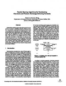
Fig. 3. Names of directed edges corresponding to a vertex whose coordinates are (6, 3).
(3) The vertex represents an obstacle (4) The vertex does not represent a source terminal, a target terminal, or an obstacle If a vertex represents a source terminal, then one (and only one) of its outgoing edges will appear in the final routing result. Moreover, none of its incoming edges will appear in the final routing result. For the example shown in Fig. 3, if vertex (6, 3) represents a source terminal, all of the following constraints must be satisfied: • E_6_3_6_4 + E_6_3_7_3 + E_6_3_6_2 + E_6_3_5_3 = 1
• • • •
E_6_4_6_3 = 0 E_7_3_6_3 = 0 E_6_2_6_3 = 0 E_5_3_6_3 = 0
Likewise, if a vertex represents a target terminal, then one and only one of its incoming edges will appear in the final routing result. Additionally, none of its outgoing edges will appear in the final result. If a vertex in a transformed graph represents an obstacle in the original routing problem, then all of the vertex’s incident edges (which include all the incoming and outgoing edges) must not appear in the final routing result. Therefore, values of E-variables for these directed edges must be set to zero. Finally, if there is a vertex which does not represent a source terminal, a target terminal, or an obstacle, then it can be passed by a wire. For each vertex of this type, the number of incoming edges must be equal to the number of outgoing edges in the final routing result. Also, the number of incoming edges appearing in the final result must be less than or equal to one. Therefore, in the example shown in the Fig. 3, the following constraints must be satisfied if vertex (6, 3) belongs to this type: •
E_6_4_6_3 + E_7_3_6_3 + E_6_2_6_3 + E_5_3_6_3 =
WCECS 2010
Proceedings of the World Congress on Engineering and Computer Science 2010 Vol II WCECS 2010, October 20-22, 2010, San Francisco, USA E_6_3_6_4 + E_6_3_7_3 + E_6_3_6_2 + E_6_3_5_3
• E_6_4_6_3 + E_7_3_6_3 + E_6_2_6_3 + E_5_3_6_3 ≤ 1 Furthermore, the above two constraints imply that the number of outgoing edges appearing in the final routing result must be less than or equal to one. IV. PREVENTION OF SUBTOURS Incorrect formulation of longest-path routing problems can result in routing solutions that contain subtours [6]. Fig. 4 illustrates a routing result which satisfies the constraints presented in Section III and the number of grid cells visited is also the maximum (31). However, it contains a subtour and the routing result is not valid. To prevent the existence of subtours in routing results, we adopt the use of U-variables; this type of variables has been used in the integer linear programming (ILP) formulation of traveling salesperson problems (TSPs) [6]. The idea of U-variables is to associate a U-variable with each vertex, so that the value of the U-variable for vertex vj is greater than the value of the U-variable for vertex vi if the directed edge vi → vj appears in the final routing result. By incorporating this method into our MILP formulation of longest-path routing problems, subtours will not appear in final routing results. Furthermore, the method will not generate an exponential number of constraints. In our MILP formulation of longest-path routing problems, the name of a U-variable is coded as u_x_y if the U-variable is associated with a vertex whose coordinates are (x, y). For each directed edge in a transformed graph, constraints regarding U-variables must be generated. For the example shown in Fig. 3, the constraint related to U-variables for the directed edge (5,3) → (6,3) is: IF ( E_5_3_6_3 = 1 ) THEN ( u_6_3
>
u_5_3 ).
However, since the relational operator “ > ” cannot be used in the standard MILP formulation, we transform the above constraint into the following: IF ( E_5_3_6_3 = 1 ) THEN ( u_6_3 – u_5_3
≥
1 ).
Note that the value of u_6_3 is now restricted to be greater than the value of u_5_3 by at least one if the directed edge exists in the routing result. This constraint can be further transformed into the following linear inequality: u_6_3 – u_5_3 + M × (1 – E_5_3_6_3)
≥ 1,
where M is a constant whose value must be sufficiently large. Therefore, when the value of E_5_3_6_3 is 1, the linear inequality becomes “u_6_3 – u_5_3 ≥ 1.” On the other hand, when the value of E_5_3_6_3 is 0, the linear inequality becomes redundant. Note that the value of E_5_3_6_3 is either 0 or 1. In the aforementioned linear inequality, since the value of M can affect the execution time of an MILP solver for solving formulated problems, it is desirable to find the minimum value of M. If the minimum value of each U-variable is defined to be zero, it can be derived that the maximum values
ISBN: 978-988-18210-0-3 ISSN: 2078-0958 (Print); ISSN: 2078-0966 (Online)
Fig. 4. An invalid longest-path routing result.
Algorithm LongestPathToMILP() Input. The description of a gridded longest-path routing problem, which includes (1) the dimension of the rectangular routing region, (2) the location of the source terminal, (3) the location of the target terminal, and (4) locations of obstacles. Output. The description of an MILP problem which corresponds to the input longest-path routing problem. 1. Transform the input longest-path routing problem into a graph (G) which contains vertices and directed edges (Section II). 2. For each directed edge in G, generate a corresponding E-variable (Section II). 3. For each vertex in G, generate a corresponding U-variable. 4. Generate a (decision) variable named “Total_Wire_Length.” 5. For each vertex in G, generate corresponding linear constraints (Section III). 6. For each directed edge in G, generate a linear constraint which is used for the prevention of subtours (Section IV). 7. Generate the linear constraint: Total_Wire_Length = (the sum of values of all E-variables) + 1. 8. Write all the generated variables and constraints into a file (e.g. in the CPLEX LP file format) which represents the formulated longest-path routing problem. Also, the value of “Total_Wire_Length” must be maximized. Fig. 5. The algorithm for transforming a gridded longest-path routing problem into an MILP problem.
of U-variables can be set to (nr*nc – nob – 1), where nr denotes the number of rows in the rectangular routing region, nc denotes the number of columns in the rectangular routing region, and nob denotes the number of grid cells that represent obstacles. That is because the number of grid cells that are not obstacles is (nr*nc – nob) in a routing problem. Thus, the maximum possible value for the difference of two U-variables is (nr*nc – nob – 1). As a result, the minimum value of M is (nr*nc – nob). In addition to the value of M, U-variables can also affect the performance of MILP solvers for finding solutions. Although U-variables can be integers, our experiments show that setting U-variables as real numbers (instead of integers) can significantly reduce the execution time of MILP solvers. V. THE ALGORITHM The algorithm for transforming a gridded longest-path routing problem into an MILP problem is detailed in Fig. 5. The value of Total_Wire_Length is computed as (the sum of values of all E-variables) + 1. In our implementation of the algorithm, in addition, output files are in the CPLEX LP file format [7]. Therefore, many different MILP solvers (e.g., IBM ILOG CPLEX, Gurobi Optimizer, and GLPK) can be used to read the files and generate solutions.
WCECS 2010
Proceedings of the World Congress on Engineering and Computer Science 2010 Vol II WCECS 2010, October 20-22, 2010, San Francisco, USA Table I. Comparison of Our Approach with Other Routing Algorithms for Solving Longest-Path Routing Problems.
Testcase Data1 Data2 Data3 Data4 Data5 Data6 Data7 Data8 Data9 Data10
Kohira [3-4] Wire Length 80 119 107 103 95 85 113 115 251 6,626
Yan [5] Wire Length 82 119 107 103 95 85 113 115 261 6,636
Transform. Time 0.22 s 0.27 s 0.27 s 0.27 s 0.27 s 0.27 s 0.27 s 0.27 s 0.45 s 1.97 s
For a given longest-path routing problem, we can observe that the number of grid cells (or vertices) is (nr*nc) and the number of directed edges is bounded by (4*nr*nc). Therefore, if we assume that n = nr*nc, the total number of variables (including E-variables, U-variables, and the variable named Total_Wire_Length) in a transformed MILP problem is bounded by O(n). Also, since a linear constraint is generated for each directed edge and at most five constraints are generated for each vertex, we can conclude that the time complexity of the proposed algorithm is linear in terms of the number of grid cells. VI. EXPERIMENTAL RESULTS The proposed algorithm for transforming longest-path routing problems into MILP problems has been implemented in Java programming language. MILP problems (or MILP problem files) generated by our program are in CPLEX LP file format [7] so that many MILP solvers can be used to find solutions. In the experiments, we used CPLEX (version 12.1) and Gurobi Optimizer (version 3.0.0) to find solutions of generated MILP problems. All the programs (including our transformation program and MILP solvers) were executed on a Linux workstation which had two Intel Xeon E5520 processors and 32 GB of RAM. Note that each of Xeon E5520 processors has four cores and is capable of executing programs with up to eight threads. Therefore, the workstation we used can run parallel MILP solvers with up to 16 threads. Table I shows the results of our approach and the comparison of our approach with other longest-path routing algorithms. Columns 2 and 3 of the table list routing results (in terms of total wire lengths) generated by the algorithms proposed in [3]–[5]. The column “Transform. Time” lists the CPU times used by our program for transforming longest-path routing problems into MILP problems. The results of using parallel MILP solvers in finding solutions of generated MILP problems are shown in the rest of the table. Note that 16 threads were used for running these solvers, and all the elapsed times were calculated as the average of multiple runs. As can be seen in Table I, compared with the algorithm proposed in [3]–[4], our approach generates better solutions for testcases Data1 and Data9. Also, compared with the algorithm proposed in [5], our approach generates a better solution for testcase Data9. In reality, our approach generates optimal solutions, i.e., longest paths, for testcases Data1 through Data9. For testcase Data10, we suspended the
ISBN: 978-988-18210-0-3 ISSN: 2078-0958 (Print); ISSN: 2078-0966 (Online)
CPLEX Wire Length Elapsed Time 1.29 s 82 119 9.83 s 107 7.05 s 103 7.69 s 95 0.92 s 85 26.58 s 113 17.23 s 115 6.88 s 263 69.75 s No Solution 29 days
Gurobi Wire Length Elapsed Time 82 1.11 s 119 4.09 s 107 4.36 s 103 5.36 s 95 0.98 s 85 139 s 113 4.34 s 115 4.45 s 453 s 263 6,495 21 days
execution of MILP solvers before they exhausted all the memory of the workstation. However, Gurobi was able to find a path whose total wire length was 6,495 in 21 days. As described in Section II, final values of E-variables, which are generated by MILP solvers, represent a solution to the original longest-path routing problem. For example, the routing result illustrated in Fig. 1(b) can be represented as: [ E_6_1_6_2=1, E_7_2_7_1=1, E_7_1_8_1=1, E_8_1_8_2=1, E_6_2_7_2=1, E_8_2_8_3=1, E_5_3_4_3=1, E_4_3_4_4=1, E_6_3_5_3=1, E_7_3_6_3=1, E_8_3_7_3=1, E_4_4_3_4=1, E_3_4_3_5=1, E_5_5_5_4=1, E_5_4_6_4=1, E_6_4_7_4=1, E_7_4_8_4=1, E_8_4_8_5=1, E_2_5_1_5=1, E_1_5_1_6=1, E_2_6_2_5=1, E_3_5_4_5=1, E_4_5_5_5=1, E_8_5_7_5=1, E_7_5_7_6=1, E_3_6_2_6=1, E_4_6_3_6=1, E_5_6_4_6=1, E_6_6_5_6=1, E_7_6_6_6=1, Total_Wire_Length=31 ]
Note that U-variables as well as E-variables whose values are zero are not listed. To measure the scalability of a parallel MILP solver in finding solutions of formulated longest-path routing problems, we used CPLEX to solve a number of formulated problems with different number of threads; the results are shown in Table II. Note that all the elapsed times were calculated as the average of multiple runs. In general, by using more threads in running the solver, less execution time is required. For the example of testcase Data8, by using 16 threads in running the solver, more than 3,700x speed-up can be achieved. While longest-path routing problems belong to the class of NP-hard [3]–[4], shortest-path routing problems can be solved in polynomial time [8]. By minimizing (instead of maxmizing) the value of Total_Wire_Length in the algorithm shown in Fig. 5, the modified approach can be used to find shortest paths. Table III shows the results of using parallel MILP solvers in finding shortest paths. As can be seen in the table, shortest-path routing problems can be solved efficiently. VII. CONCLUSION We proposed an MILP formulation to gridded longest-path routing problems. The proposed algorithm is capable of transforming a longest-path routing problem into an MILP problem. The algorithm is efficient since the time complexity is linear in terms of grid cells in the original routing problem. After a longest-path routing problem has been transformed into an MILP problem, parallel MILP solvers can be used to
WCECS 2010
Proceedings of the World Congress on Engineering and Computer Science 2010 Vol II WCECS 2010, October 20-22, 2010, San Francisco, USA Table II. Elapsed Time of Using CPLEX in Solving Longest-Path Routing Problems with Different Number of Threads.
Testcase Data1 Data2 Data8 Data9
1 thread 36.39 s 642.74 s 25,491.82 s 10,885.65 s
1x 1x 1x 1x
2 threads 28.06 s 1.3x 96.05 s 6.7x 469.27 s 54.3x 6,509.02 s 1.7x
CPLEX 4 threads 9.58 s 3.8x 45.30 s 14.2x 100.90 s 252.6x 5,081.46 s 2.1x
8 threads 4.67 s 7.8x 16.87 s 38.1x 19.51 s 1307x 3,092.72 s 3.5x
16 threads 1.29 s 28.2x 9.83 s 65.4x 6.88 s 3,705x 1,431.35 s 7.6x
Table III. Elapsed Time of Using MILP Solvers in Finding Solutions to Shortest-Path Routing Problems.
Testcase Data1 Data2 Data3 Data4 Data5 Data6 Data7 Data8 Data9 Data10
CPLEX Wire Length Elapsed Time 9 0.01 s 22 0.02 s 12 0.01 s 12 0.01 s 12 0.01 s 12 0.01 s 12 0.01 s 12 0.02 s 8 0.03 s 153 3.83 s
find solutions. As a result, computational power of multi-core processors can be exploited. Although the performance of our approach cannot compete with a number of existing routing algorithms, the approach can be used to find optimal solutions or to prove optimality of solutions. Moreover, since high degrees of scalability can be achieved, the proposed approach can be attractive when a computer which contains many processor cores is available. REFERENCES [1] M. M. Ozdal, and M. D. F. Wong, “A length-matching routing algorithm for high-performance printed circuit boards,” IEEE Transactions on Computer-Aided Design of Integrated Circuits and Systems, vol. 25, no. 12, December 2006, pp. 2784-2794. [2] M. M. Ozdal, and M. D. F. Wong, “Algorithmic study of single-layer bus routing for high-speed boards,” IEEE Transactions on Computer-Aided Design of Integrated Circuits and Systems, vol. 25, no. 3, March 2006, pp. 490-503.
ISBN: 978-988-18210-0-3 ISSN: 2078-0958 (Print); ISSN: 2078-0966 (Online)
Gurobi Wire Length Elapsed Time 9 0.02 s 22 0.04 s 12 0.03 s 12 0.03 s 12 0.03 s 12 0.03 s 12 0.04 s 12 0.03 s 8 0.05 s 153 11.42 s
[3] Y. Kohira, S. Suehiro, and A. Takahashi, “A fast longer path algorithm for routing grid with obstacles using biconnectivity based length upper bound,” IEICE Transactions on Fundamentals of Electronics, Communications and Computer Sciences, vol. E92-A, no. 12, December 2009, pp. 2971-2978. [4] Y. Kohira, S. Suehiro, and A. Takahashi, “A fast longer path algorithm for routing grid with obstacles using biconnectivity based length upper bound,” in Proceedings of Asia and South Pacific Design Automation Conference, 2009, pp. 600-605. [5] J.-T. Yan, M.-C. Jhong, and Z.-W. Chen, “Obstacle-aware longest path using rectangular pattern detouring in routing grids,” in Proceedings of Asia and South Pacific Design Automation Conference, 2010, pp. 287-292. [6] W. L. Winston, and M. Venkataramanan, Introduction to Mathematical Programming, Thomson Learning, Inc., 2003. [7] IBM, IBM ILOG CPLEX V12.1 - File Formats Supported by CPLEX, 2009. [8] C. Y. Lee, “An algorithm for path connections and its applications,” IRE Transactions on Electronic Computers, September 1961, pp. 346-365.
WCECS 2010