of string

Durham E-Theses

Aspects of plane waves and Taub-NUT as exact string theory solutions Svendsen, Harald Georg

How to cite:

Svendsen, Harald Georg (2004) Aspects of plane waves and Taub-NUT as exact string theory solutions, Durham theses, Durham University. Available at Durham E-Theses Online: http://etheses.dur.ac.uk/2947/

Use policy

The full-text may be used and/or reproduced, and given to third parties in any format or medium, without prior permission or charge, for personal research or study, educational, or not-for-prot purposes provided that: • a full bibliographic reference is made to the original source •

a link is made to the metadata record in Durham E-Theses

• the full-text is not changed in any way The full-text must not be sold in any format or medium without the formal permission of the copyright holders.

Please consult the full Durham E-Theses policy for further details.

Academic Support Oce, Durham University, University Oce, Old Elvet, Durham DH1 3HP e-mail: [email protected] Tel: +44 0191 334 6107 http://etheses.dur.ac.uk

Aspects of plane waves and Taub-NUT as exact string theory solutions Harald Georg Svendsen

A copyright of this thesis rests with the author. No quotation from it should be published without his prior written consent and information derived from it should be acknowledged.

A thesis presented for the degree of Doctor of Philosophy

- 6 DEC 2004 Centre for Particle Theory Department of Mathematical Sciences University of Durham England September 2004

Aspects of plane waves and Taub-NUT as exact string theory solutions Harald Georg Svendsen Submitted for the degree of Doctor of Philosophy September 2004 Abstract This thesis is a study of some aspects of string theory solutions that are exact in the inverse string tension a/, and thus are valid beyond the low-energy limit. I investigate D-brane interactions in the maximally supersymmetric plane wave solution of type lib string theory, and study the fate of the stringy halo surrounding D-branes. I find that the halo is like in flat space for Lorentzian D-branes, while it receives a non-trivial modification for Euclidean D-branes. I also comment on the connection between Hagedorn temperature and T-duality, which motivates a more general study of T-duality in null directions. I consider such transformations in a spinning D-brane solution of supergravity, and find that divergences in the field components associated with null T-dualities are invisible to string and brane probes. I also observe that there are closed timelike curves in all the T-dual solutions, but that none of them are geodesics. The second half of the thesis is an investigation of the fate of closed timelike curves and of cosmological singularities in an exact stringy Taub-NUT solution of heterotic string theory, and in a rotating generalisation of it. I compute the exact spacetime fields, using a description in terms of a gauged Wess-Zumino-NovikovWitten model, and find that the a/ corrections are mild. The key features of the Taub-NUT geometry persist, together with the emergence of a new region of space with Euclidean signature. Closed timelike curves are still present, which is interpreted as a sign that they might be a natural ingredient in string theory, for instance in pre-Big-Bang cosmological scenarios.

Declaration The work in this thesis is based on research carried out at the Centre for Particle Theory, the Department of Mathematical Sciences, University of Durham, England. No part of this thesis has been submitted elsewhere for any other degree or qualification and it is all my own work unless referenced to the contrary in the text. Parts of the work presented in this thesis have been published as research papers written in collaboration with my supervisor, Prof. Clifford V. Johnson. These are refs. [1,2], and correspond to chapters 3 and 6. Chapters 2 and 5 are mostly reviews of already known material, while chapters 4 and 7 contain new unpublished results based on my own research.

Copyright© 2004 by Harald G. Svendsen. The copyright of this thesis rests with the author. No quotations from it should be published without the author's prior written consent and information derived from it should be acknowledged. iii

Acknowledgements First of all, I am very grateful to Prof. Clifford V. Johnson who has been my supervisor, and a tremendous source of inspiration and knowledge throughout my time as his student. Thank you. I also owe many thanks to my colleagues, Emily Hackett-Jones and Anton Ilder-

ton for answering many of my odd questions, and also Matthew Killeya and Gavin Probert for enlightening discussions on both scientific and other topics. You have all made office days very enjoyable. Many thanks to Profs. Hallstein H0gasen and Ulf Lindstrom for helping me to get started with my doctoral studies, and to Drs. Chong-Sun Chu, Douglas Smith, Simon Ross, Laur Jiirv, and James Gray for help at various stages. Thanks also to all other members of the maths department at Durham University for providing a very stimulating and friendly atmosphere. I thank Norway for a doctoral student fellowship without which I could not have

pursued these studies, and Britain for an Overseas Research Student Award. I am also grateful for financial support from the University of Durham, through a Nick Brown memorial bursary and other travel grants. Thanks to the high-energy physics group at the University of Southern California for hospitality. I have enjoyed my time in Durham - the hills, the trees, the paths and buildings

surrounding me have kept me happy. But more so because of my friends. Thank you all. Especially Grace (for all the fun) and the other "UN house" people: Aris, Karen, Manuel, and Maria. Thanks also to Durham University Fencing Club and Graduate Society Boat Club for many happy times. The work towards the completion of this thesis started in many ways long before I came to Durham. And ever since my first day in primary school, I have had

excellent teachers who have inspired me and encouraged me. A great part of the achievement manifested by this thesis belongs to you. Finally, huge thanks to my parents, Gerd Marit and Johan, and to my siblings. Through your persistent encouragement and faith in me you have helped me much more than you know. iv

Contents Abstract

ii

Declaration

iii

Acknowledgements

IV

1 Introduction

1

1.1

State of string theory .

1

1.2

Context and motivation

3

1.3

Outline and summary of results

4

2 Plane wave solutions 2.1

2.2

2.3

2.4

6

Strings in plane waves

7

2.1.1

Quantisation

.

2.1.2

Plane waves as a Penrose-Giiven limit.

7

The AdS/CFT correspondence and its BMN limit

9

2.2.1 2.2.2

AdS/CFT correspondence Dictionary ..

9

12

2.2.3

BMN limit ..

13

D-brane interactions 2.3.1

D-branes in plane waves

2.3.2

Interactions in fiat space

14 14 16

2.3.3

Interactions in plane waves .

18

Hagedorn temperature and T-duality

3 D-brane-anti-D-brane interactions in plane waves 3.1

3.2

8

21

Introduction . . . . . . . . . . . .

26 26

3.1.1

Superstrings in fiat space .

27

3.1.2

Plane waves

30

The Interaction ..

30 v

Contents

3.3

4

vz

3.2.1

The Amplitude and Potential . . . .

31

3.2.2

Divergences, Tachyons, and the Halo

32

Summary . . . . . . . . . . . . . . . . . . .

36

T-dualities in null directions, and closed timelike curves

37

4.1

Introduction

37

4.2

T-dualities .

40

4.2.1

T-dual along z direction

41

4.2.2

T-dual along ¢ 1 direction .

41

4.2.3

T-dual along both

4.3

4.4

(h

and z directions.

42

Probe calculations in T q, 1 z-dual solution . . . .

44

4.3.1

Fundamental string coupled to B-field

44

4.3.2

D1-D5-brane probe

46

4.3.3

D3-brane probe ..

47

Closed timelike curves 4.4.1

. .

48

CTCs and geodesics

50

Discussion . . . . . . . . . .

52

5 Wess-Zumino-Novikov-Witten models

54

4.5

5.1

WZNW models . . . . . . . . . . . . .

54

5.2

Coset models as gauged WZNW models

57

5.3

Exact spacetime fields from coset models

59

5.3.1

The Exact Effective Action

60

5.3.2

Computation of the Exact Effective Action .

61

5.3.3

Extracting the Exact Geometry

64

5.3.4

Example: A 2D black hole

67

Heterotic coset models . . . . . .

69

5.4.1

Abelian bosonisation . . .

70

5.4.2

Non-Abelian bosonisation

71

5.4.3

Re-fermionisation . . . . .

72

A deformation of a charged 2D black hole

74

5.4

5.5

6

...

High energy corrections in a stringy Taub-NUT spacetime

78

6.1

Introduction and Motivation . .

79

6.2

Stringy Taub-NUT . . . . . . .

82

6.3

Exact Conformal Field Theory .

87

6.3.1

The Definition. . . . . .

87

6.3.2

Writing The Full Action

88

6.3.3

Extracting the Low Energy Metric

90

Contents 6.4

6.5

vn

Exact spacetime fields

. . . . . . . . .

91

6.4.1

Computations . . . . . . . . . .

92

6.4.2

Properties of the Exact Metric .

96

Discussion . . . . . . . . . . . . . . . .

98

7 High energy corrections in a stringy Kerr-Taub-NUT solution 7.1

Exact conformal field theory

. 102

7.2

Low-energy limit . . . . . .

104

7.3

Exact metric and dilaton . .

105

7.3.1

106

7.4

8

102

Properties of metric .

Discussion

109

Conclusion

111

Appendices

114

A Definition of functions

114

A.1 Generalised Jacobi functions

114

A.2 Deformed theta functions . .

116

B Summary of thesis for laymen

117

B.1 Norwegian translation Bibliography

. 119

123

List of Figures 2.1

D-brane interactions and open/closed duality.

15

3.1 Cylinder diagram 3.2 Stringy halo . . .

30 35

6.1 6.2 6.3 6.4

84 86 97 98

Various regions of the classical stringy Taub-NUT geometry Throat region of the Taub-NUT geometry . . . . . . . . . Various regions of stringy Taub-NUT for arbitrary k . . . . Various regions of stringy Taub-NUT for lowest possible k

7.1 Horizon and ergosphere of stringy Kerr-Taub-NUT geometry. 7.2 Singularities in stringy Kerr-Taub-NUT geometry, small T 7.3 Singularities in stringy Kerr-Taub-NUT geometry, large T . . .

Vlll

. 107 . 108 . 109

List of Tables 2.1

Possible D-brane configurations in plane waves . . . . . . . . . . . . . 15

lX

Chapter 1 Jrntrod uctlion 1.1

State of string theory

String theory appeared first [3-6] as a theory to explain strong nuclear interactions. It was put aside as such by the successful Quantum Chromo Dynamics (QCD) theory. However, it became clear that string theory is a theory of a much greater potential [7]: a theory of quantum gravity. The theory as far as it was understood had various problems, and much of the initial excitement went away. But a decade later a new breakthrough was made with the discovery of anomaly cancellations [8], often referred to as the first string revolution. Since then, much work has been done in string theory, with a number of remarkable advances. One of the most important came in the mid-nineties with the discovery of D-branes [9], setting off the second

string revolution. Insight gained over the last decade or so has taught us that the different superstring theories (type I, type IIA and B, heterotic E 8 x E 8 and S0(32)) are really just different perturbative limits of the same underlying theory, the M-theory. But as clear as this is, it is equally unclear what is the proper formulation of this mysterious theory. A summary of my thesis for laymen is given in appendix B. An excellent introduction to string theory for non-physicists is ref. [10]. Textbooks on string theory are refs. [11-15]. Some other, briefer introductions are refs. [16-19].

String theory and the real world In many respects it might be more fruitful to think of string theory as a framework for theoretical physics, rather than as one particular theory about the fundamental particles and their interactions. String theory has and continues to teach us a lot about connections within theoretical physics and indeed mathematics. For 1

1.1. State of string theory

2

example, string theory has through various dualities opened up windows to exact non-perturbative phenomena in gauge theory. This makes string theory highly interesting to study, independently of whether it is an accurate description of elementary particles and gravity as manifested in our world. So there are several strong, but purely theoretical motivations for doing string theory. From this point of view, the research is not so much about understanding the universe per se, but about understanding our theories about the universe. By understanding them better, we can more easily extend them, or correct them where they turn out faulty or inconsistent. Nevertheless, much work is also being undertaken to try and relate string theory to the observable world. Phenomenology is the bridging discipline between theoretical and experimental physics, and over the last few years the new field of string phenomenology has evolved. The central questions are: What can we deduce from string theory about the observable world? What constraints do our experimental results put on string theory? Of utmost interest is the question of how to reproduce the Standard Model from string theory. In the "old days" (before mid-nineties), heterotic strings were the favourite tool to achieve low-energy dynamics in four dimensions that resemble our world. Nowadays, type II theories with D-branes are the more popular ones - but with the understanding that all the superstring theories are anyway related by various dualities. Another area where there are real prospects for communication between string theory and observations is cosmology. Recent years have seen remarkable progress in astronomy, with increased accuracy in observational data. These put strong constraints on various fundamental parameters. They also seem to tell us that the vast majority of the energy in the universe is of a still unknown sort called "dark energy". String theory should predict these data if it is to be taken seriously as a quantum gravity theory. Moreover, the energy scales needed to test string theory seem to be far too high to be achievable in a laboratory on Earth, so data taken from (indirect) observations of extreme phenomena like the first moments of the universe, and of black holes might be our best chance as a test ground for string theory. Having said this, certain aspects of string theory should also be testable in the next generation accelerators. 1 The most important amongst these is probably supersymmetry, which can be viewed as a prediction from string theory. If supersymmetry is not detected, it will be an embarrassment, but certainly not the end of string theory. 1

The Large Hadron Collider at CERN is to be operational in 2007.

1.2. Context and motivation

3

Some open problems

One of the big problems in string theory is the vacuum degeneracy: There is an enormously large number of different ways to arrive at low-energy dynamics in four dimensions, and no good principle to tell us which is the right one. This is related to the cosmological constant problem: Why is it that the cosmological constant is so small, yet non-zero and positive? The vacuum degeneracy is also at the heart of the problems with making experimental predictions from string theory. The problem is not that string theory gives wrong predictions, but rather that it does not single out any one of the large number of possibilities. On a conceptual level, a problem with string theory today is that it does not really have a proper definition. The string theories are only defined perturbatively, and although there is strong evidence of the existence of an underlying theory, theMtheory, its proper formulation is still unknown. These and other difficulties usually makes it hard to do calculations in the full string theory. One way to get a much more tractable theory is to restrict ourselves to the low-energy regime where the inverse string tension a'

-t

0. Most explicit calculations in string theory have been

done in this limit. This thesis is a study of some aspects of string theory beyond this low-energy limit. There are of course many more open questions and unsolved problems in string theory, but it is a much too involved task to discuss them all here.

1.2

Context and motivation

Much is known about string theory and solutions of the string theory equations in the low-energy a'

-t

0 regime, which is the supergravity limit. The title of this thesis

includes the words "exact string theory solutions", and by that I mean solutions that go beyond this limit, and are valid solutions of string theory to all orders in

a', including non-perturbative effects. Note that the supergravity limit sends the string length ls =

#

to zero, so effectively it treats the strings as point particles

and ignores the oscillations of the strings. This gives a field theory of particles, but it nevertheless contains stringy corrections through the presence of extra fields, like the antisymmetric B-field and the Ramond-Ramond fields. A common feature of supergravity solutions, which I will discuss in this thesis, is the existence of closed timelike curves (CTCs). These are also there in General Relativity, and represent time-loops in the spacetimes, leading to problematic paradoxes and divergences in physical quantities like the stress-energy tensor. It is a common belief that the CTCs and the problems associated with them disappear in

1. 3. Outline and summary of results

4

the full string theory. But due to the lack of string models where CTCs can be studied by explicit calculations, this has mainly remained a speculation. It is clear that the string oscillations cannot always be ignored, and it is interesting to study string theory models where we can also take into account that the strings are not pointlike objects. However, the scarcity of exact classical solutions where this is possible is an obstacle to a better understanding of string theory. There are only two classes of solutions known to be exact in o/. The first is the class of plane-wave backgrounds, or more generally, solutions with a covariantly constant null Killing vector. These are exact solutions which receive no o/ corrections due to special properties of the background. The second is the class of gauged Wess-Zumino-Novikov-Witten (WZNW) models. These are worldsheet conformal field theories which have a Lagrangian description which makes it relatively easy to deduce the quantum effective action, and thereby the exact background fields. In addition, Minkowski space is an exact string theory solution, and also orbifolds of Minkowski space are. These are exact because the curvature is zero, and therefore all o:' corrections vanish to all orders. An example [20] of such an orbifold is the Milne space. For a review of exact solutions of closed string theory see ref. [21]. In this thesis I will study examples from each of the two primary classes of exact solutions. The first is a parallel plane wave with non-zero Ramond-Ramond (RR) flux. The aspect of it that I am going to investigate concerns D-brane-anti-D-brane interactions, in particular the so-called stringy halo surrounding the D-braries. The gauged WZNW model examples I will study are a stringy Taub-NUT space and a generalisation of it with rotation. I will compute the o:' corrections to the spacetime fields (which have not been computed before), and then study some properties of the solution.

1.3

Outline and summary of results

In chapters 2 and 3 I will study D-branes and D-brane interactions in a plane wave background. D-branes are at present well understood in a flat spacetime background, but rather poorly understood in more general backgrounds. Being a background where the study of D-branes is tractable, the plane waves are therefore of great interest in this respect. D-branes are known to be surrounded by a stringy halo, which marks the edge of the region within which tachyon condensation occurs. The goal of the first part of my thesis is to investigate this halo in the plane wave background, and study how it differs from what is known for D-branes in flat spacetime.

1. 3. Outline and summary of results

5

We shall see that the there is an important difference between Lorentzian Dbranes and Euclidean D-branes. The former have a stringy halo just like in the flat space, while the latter have a halo deformed by the plane wave parameter f.L. Chapter 4 picks up on an observation regarding thermal strings in plane waves: T-dualties in null or timelike directions might be relevant for understanding the Hagedorn temperature. In this chapter I will study another system to gain more insight into the general issue of T-dualities in null and timelike directions.

An

asset of the model I will consider is that it contains a parameter which serves as a regulator, allowing the T-duality to become null or timelike in a controlled way. I find that probe calculations give reasons to believe that null or timelike Tdualities do not really represent a problem in the string theory, although components of the supergravity fields become divergent. We will also observe closed timelike curves in this model, persisting the T-dualities, and I argue that none of these are geodesics. The observation of closed timelike curves in supergravity solutions, and the wish to understand their role in string theory is part of the motivation for the work of the subsequent chapters 5, 6 and 7. I will do this by studying two examples from the second class of exact string theory solutions. These are gauged Wess-ZuminoNovikov-Witten models, associated with heterotic coset model constructions. I will present the general techniques required to deduce the exact spacetime fields (chapter 5), and then study a stringy Taub-NUT solution (chapter 6) and its rotating generalisation (chapter 7). Of special interest is the issue of CTCs in the resulting spacetimes. The corresponding supergravity solutions have been known to have CTCs, and these models provide exactly the kind of computational control we want for an investigation of the fate of CTCs in full string theory. Another motivation for investigating these models is that they contain cosmological regions with a Big Bang and a Big Crunch, thereby facilitating a study of cosmological singularities in string theory. The conclusion is that the string theory modifications are mild and do not modify the spacetime in such a way that the closed timelike curves disappear. This is a hint that although problematic in General Relativity, the existence of closed timelike curves might not necessarily be a problem in string theory.

Chapter 2 Plane wave solutions Plane wave spacetimes are exact solutions of superstring theory which may or may not come equipped with Neveu-Schwarz-Neveu-Schwarz (NSNS) or RamondRamond (RR) flux. In this and the next chapter, I will focus on plane waves with a non-trivial five-form RR field [22]. They are very interesting for various reasons. First of all, they are tractable systems which are exact to all orders in ci, and therefore very useful models in which to study string theory in RR backgrounds, which has been a poorly understood subject. Moreover, the parallel plane wave (pp-wave), which has constant RR flux, contains 32 supersymmetries, which is the maximum number. This puts it alongside Minkowski space and the AdS5 x 5 5 solutions as the only maximally supersymmetric solutions of string theory. In fact, the pp-wave can be found as a Penrose-Giiven limit of AdS5 x 5 5 , and this is another highly attractive asset of it, as I will come back to. It means that the plane wave plays part in string/gauge theory dualities inherited from the AdS/CFT correspondence via the Penrose-Giiven limit. To find the spectrum of states we have to rely on light-cone gauge, which then makes the task easy. But that gauge also has some awkward features. It means that the worldsheet theory is not conformally invariant since the worldsheet fields are massive. So e.g., string interactions are hard to evaluate. However, in this and the next chapter I will study static interactions between pairs of D-branes, which is an easier problem. I will start with a review of string theory in the plane wave background. Then I will briefly describe the AdS/CFT correspondence, and the limit of it that is relevant for plane wave physics. The main part of the chapter is a general discussion of Dbrane interactions and the open/closed duality. This will set up the notation, and serve as background for the discussion in chapter 3. Finally, I will demonstrate the existence of a Hagedorn temperature and its relation to the self-dual radius under 6

2.1. Strings in plane waves

7

aT-duality transformation.

2.1

Strings in plane waves

The parallel plane wave spacetime is a maximally supersymmetric solution of string theory with the metric and RR flux given as [22]: 4

ds 2

=

2dx+dx-- p, 2x 2(dx+) 2 +

8

L dxidxi + L dxidxi , i=l

i=5

(2.1)

8

F+l234 = F+s678 = 2p, ,

x2 = I:xixi' i=l

It yields an exactly solvable string model [23] (in light-cone gauge). The metric has

an S0(8) symmetry which is broken to S0(4)

X

S0(4)

X z2

by the presence of the

RR-field.

2.1.1

Quantisation

The presence of the RR flux in the plane wave solution (2.1) makes it highly nontrivial to formulate string theory in this background. But if we ignored this problem and tried to write down a standard nonlinear sigma model,

even the bosonic sector would be problematic in a general covariant gauge, due to the non-trivial spacetime metric GJ.J.v· However, if we choose a light-cone gauge defined by relating worldsheet time T to x+ via x+ = 2na'p+T, where p+ is the

+ component

of spacetime momentum, the bosonic part simplifies and essentially

gives a free massive theory. Remarkably, the light-cone gauge also allows us to write down the contribution from the fermionic sector [23]. This is done using the Green-Schwarz formulation of superstrings, rather than the more conventional Ramond- Neveu-Schwarz formulation. The resulting Lagrangian is (2.3) where i

=

1, ... , 8 is a spacetime index, a

= 1, ... , 8 is a spinor index, and the

mass parameter is NI = 2nolp+ p,. The matrix 11 is a product of gamma matrices,

2.1. Strings in plane waves

8

IT= 1 11 21 3 1 4 , and the spinors

sa and !Ja are left- and right-moving 50(8) spacetime

spinors respectively. It is apparent from the Lagrangian (2.3) that this is a model of eight free massive

bosons and fermions, and should therefore be easy to quantise.

The light-cone

(closed string) Hamiltonian is 00

2p+ H

=

I:

(2.4)

/wk/Nk>

k=-oo

where Nk is the total (bosonic plus fermionic) number operator, and wk is the oscillator frequency for mode k. A notable difference from flat space is that also the zero-modes are oscillators in the plane wave case. Upon quantisation, the Hamiltonian (2.4) gives the complete spectrum for the strings in the plane wave background, and the model is therefore said to be an exactly solvable string theory model.

2.1.2

Plane waves as a Penrose-Giiven limit

An interesting feature of the plane wave solution (2.1) is that it can be found as a particular scaling limit of AdS5 x S 5 [24]. This is the Penrose-Giiven limit [25, 26], which essentially blows up the geometry of any spacetime around a chosen null geodesic, while scaling the various other fields such that they also survive the limiting procedure. Such limits always result in plane wave spacetimes, albeit more general ones than the parallel plane wave (pp-wave) solution (2.1) that I consider in this thesis. How to take this limit can be formulated in general terms, but in the case of AdS5 x S 5 a rather direct and simple procedure is possible. 1 The AdS5 x S 5 metric

can be written

where R is the radius of curvature, and is the same for both parts of the metric. Introduce light-cone coordinates

x± = 0.('1/J ± t). X

J.LR'

Then make the rescalings

(2.6)

with an arbitrary mass parameter f-l, and take the limit R--+ oo. This "blows up" 1

A calculation demonstrating how the limit can be taken in the more general case is found in ref. [27).

2.2. The AdS/CFT correspondence and its BMN limit the region close to the null-geodesic parameterised by

9

x+.

The resulting metric is

The AdS5 x S 5 spacetime as a solution of type IIB string theory also comes with a RR flux (2.8) where E(M) is the natural volume form on the manifold M. In the above scaling limit this becomes

Hence the Penrose-Giiven limit of the AdS5 x 8 5 solution of type liB string theory gives exactly the plane wave solution (2.1). With the AdS/CFT correspondence in mind (see next section), this is very interesting. We know that there is a duality between string theory on AdS5 x 8 5 and a certain conformally invariant gauge theory. However, one problem with the AdS/ CFT correspondence is that the spectrum of states is unknown for string theory in AdS5 x S 5 , so that for practical computations we are restricted to the supergravity limit. But we have just seen that the plane wave background is tractable even for the full string theory, and since it is related to AdS5 x 8 5 by a scaling limit, there is good reason to be excited: There ought to be a dual limit on the gauge theory side, giving a correspondence between string theory on plane waves and some sector of a gauge theory. Such a correspondence indeed exists (28], and is often referred to as the BMN limit of the AdS/CFT correspondence. It opens up a whole new window to string/ gauge theory dualities, and has been a field of active research since its discovery.

2.2

The AdS/CFT correspondence and its BMN limit

2.2.1

AdS /CFT correspondence

The AdS/CFT correspondence (29-31] is a realisation of quite an old idea (32] that there is a connection between large N gauge theories and string theories. It is also a realisation of the holographic principle that a gravitational theory in a number of

2.2. The AdS/CFT correspondence and its BMN limit

10

dimensions is equivalent to a non-gravitational theory in less dimensions. In short, the AdS/CFT correspondence states: Type IIB string theory on AdS5 x S5 with integer 5-form flux N across the S 5 is dual to

N = 4 supersymmetric conformal field theory ( CFT)

in 3+1 dimensions with gauge group U(N). Recall that type IIB string theory has D-branes of odd spatial dimensions. To derive a weaker form of the correspondence, consider an integer number N of coincident D3 branes in fiat 10-dimensional Minkowski space. There are two different low-energy descriptions of this system, and it is the equivalence of these descriptions which gives the above correspondence. First, however, let me clarify what limit we shall be working in: Remember that the low-energy approximation of string theory is obtained by sending c/ --. 0. We want to arrive at a sensible gauge theory where certain quantities survive the limit, e.g. the energy of a "W boson". Now, consider a brane located away a distance r from the N coincident D3-branes. A string stretched between this brane and the brane-stack represents such a "W boson" with an energy= tensionxlength""

~'

= u.

So, this is a quantity we want to keep fixed, which means we have to send r --. 0. Description one

The system we consider can be described by open and closed

strings. The D3-branes represent excitations of open strings, while the bulk geometry represents excitations of closed strings. In addition, there are interactions between the brane and the bulk. In the limit a

-->

0, r

-->

0,..; = fixed, the open a

string excitations are described by a gauge theory living on the brane worldvolume. To be more specific, it is an N = 4 supersymmetric U(N) conformally invariant gauge theory (CFT) in 3+1 dimensions. The gauge coupling is g~M = 27rg 8 , where 9s is the string coupling.

Now, consider the closed string excitations in the bulk. By taking the low-energy limit a'

-->

0, we are left with the massless modes only, that is, type IIB supergravity.

The interactions between these two sectors are suppressed in the limit. For this reason it is referred to as the decoupling limit. This decoupling of the open and closed sectors is crucial for proving the weak correspondence. In summary, this limit means S=

Description two

Sbrane

+ Sbulk + Sint

-->

ScFT

+ Sflat space sugra·

(2.10)

Another way to view the system of N coincident D3-branes is

by realising that it corresponds to a solitonic solution of type IIB supergravity. The

2.2. The AdS/CFT correspondence and its BMN limit

11

branes warp the geometry, and are sources for a RR 5-form field strength F5 . The bosonic part of this solution is given as

ds 2 =H(r)-~ (-dt 2 + dxi

Fs =(1 + *)dC4,

+ dx~ + dx~) + H(r) ~ (dr 2 + r 2 dD~),

C4 = dt 1\ dx1

1\

dx2

1\

(2.11)

dx 3 ,

e21> =g2 s'

where

(2.12) It is easy to see that the above solution has a horizon for r = 0, so the limit r

-+

0

means that we zoom in on the near horizon geometry. Doing this with u = .; fixed a g1ves

(2.13) where a factor of a/ has been absorbed into the coordinates t and

Xi·

This geometry

5

is AdS5 x 5 (in local coordinates), with the same radius of curvature R for both the anti-de Sitter part and of the 5-sphere. Again there is a decoupling, now between this near-horizon region and the asymptotic region. As r

-+

oo, the solution (2.11) gives just fiat Minkowski space, and so

this asymptotic region is described by liB supergravity on fiat space. There are no interactions left in this limit, since there would be an infinite redshift for a signal going from the near horizon region to the asymptotic region. In summary, the limit in this description amounts to

S =

Swarped 03-brane geometry

-+

S AdS su~a + Sftat space sugra·

(2.14)

Comparing the two descriptions, we see that in both cases we have a part described by supergravity in fiat space. Identifying these, we are led also to identify the two other terms. Hence we identify 4D U(N) gauge theory (which is a CFT) with type

liB supergravity in AdS5 x 5 5 background. This gauge theory is a rather special one in that it is has N = 4 superconformal symmetry. The bosonic part of the Lagrangian is

(2.15) where

Ff-Lv

is the gauge field strength, and ¢i are six real scalars. The fields belong to

a supermultiplet which transforms in the adjoint of U(N). TheN= 4 superalgebra

2.2. The AdS/CFT correspondence and its BMN limit

12

is very constraining, and determines the Lagrangian almost uniquely. The only freedom is in the gauge group and the coupling

gyM

which is a true (non-running)

parameter since the ,8-function vanishes due to the conformal symmetry.

Validity of descriptions The supergravity approximation to string theory can only be trusted when curvatures are small (i.e., radius of curvature is large compared to string length #). From (2.12) it is clear that g 8 N then has to be large. In addition, the above descriptions have only taken into account tree level diagrams, so loop contributions should be suppressed - in other words, we need g 8 small. All in all, we can do calculations on the string theory side (and trust the result) when g8 N

»

1,

N»l.

(2.16)

On the gauge theory side, the effective coupling is the 't Hooft coupling A. = g~ MN = 2ng8 N. So the regime where the supergravity can be trusted corresponds

to the strong 't Hooft coupling regime. The gauge theory on the other hand, is well understood only in the weak coupling. Hence, rather than a simple equivalence between two well-known theories, this is a strong/weak duality. As "derived" here, this duality is between supergravity and gauge theory in the large N limit. And in this limit the correspondence is well established. However, the Maldacena conjecture (which is much harder to verify) states that it is valid for arbitrary N. It is this stronger form of the duality which usually goes under the name of the AdS/ CFT correspondence. Beyond the large N limit, the supergravity approximation is not valid anymore, and we have to work with the full string theory. But as mentioned already, how to do string theory calculations in the AdS5 x S 5 background is not well understood yet. One of the reasons that string theory on AdS5 x S 5 has remained an unsolved problem is the presence of RR flux. Some reviews on the AdS/CFT correspondence are refs. [33-35].

2.2.2

Dictionary

The AdS/CFT correspondence says that string theory on AdS5 x S 5 is equivalent to a conformally invariant gauge theory in four fiat dimensions with

N = 4 SUSY.

One simple check of this correspondence is to compare the symmetries: The 50(6) isometry group of S 5 is the R-symmetry group in the gauge theory, and SO( 4, 2) isometry group of AdS5 is the conformal group in four dimensions.

2.2. The AdS/CFT correspondence and its BMN limit

13

The correspondence relates partition functions of the two theories: (2.17) where the source

IPb of the appropriate operator Oi on the gauge theory side is

identified with the boundary value of the supergravity field 0

"'

_2

72

B(a)

e

T2

,

(2.48)

(71,72)

where Jl.![ = 2ncip+/-L, and B(a) is some factor that is independent of T 1 and

72,

but

2.4. Hagedorn temperature and T-duality

24

does depend on a. The "deformed theta functions"

z{%:o and ztt) are defined in

appendix A.2. The partition function now diverges if

2ab O

the sets P± are defined in appendix A.l. For our

discussion, the only important fact about the function G(t) is that its behaviour at large and small t is such that generically, the amplitude is convergent. That A is finite as t --t 0 follows from the fact that small t is the closed string IR limit, where this amplitude should reproduce simple low energy field theory results for massless exchange at tree level. The t --t oo limit is also well behaved generically, since this is the open string IR limit, which is fine - away from special circumstances which will not show up in the oscillator contributions since their energies are higher than the lowest lying states. In fact, it is clear that G(t) --t 1 as t --too, and so whether

A is finite as t --t oo depends on the sign of the exponent Z, which controls those lowest lying states. The divergence for negative Z is related to the lowest lying states becoming tachyonic at this point, as is most familiar in the RNS formulation in the fiat spacetime background (see section 3.1.1.) Let us write everything in terms zi, the separation between the branes in the eight directions xi, defined by y~ = y~ + zi. The expression for Z then becomes (recall c: = 0 for p = 1 case, and c: = 1 for p = -1 case)

Z(m, y1, z)

m7r [ 1 2 h( ) (z +a) , 2 41r a tan m1r

= -

. 'tE

tanh(m1r) + _ m1r

2]

z z - b ,

(3.15)

where I have defined:

a=

cosh(m1r)- 1 Y1 cosh(m1r) ' (3.16)

For the Lorentzian p = 1 case, these parameters simplify further in the t --t oo limit of interest. Since for fixed z+ the large t region corresponds to small p+ (this follows from equation (3.7), or on general grounds from the operator definition of

34

3.2. The Interaction

the amplitude), we see that m-. 0 in all of these expressions, and so we obtain: 1 z -----+ -2(z2 41f o:'

21f2 o:') '

(3.17)

This is in fact the same expression we would obtain from the equivalent flat space computation, which simply has m = 0 throughout, and so we recover the well known [48] divergence at separation given by z~ = 21f 2o:'. In fact, the result ought to be present for all Lorentzian branes, as the relevant amplitude can be defined directly in the open string light cone gauge. Intuitively, we are looking for a result in the open string IR limit t -. oo, which (from equation (3. 7)) corresponds top+

-t

0.

But the parameter upon which any new physics can depend ism= 21ro:'p+ f-1, which vanishes in the limit. So there is no new physics. For the Euclidean p = -1 case, the situation is very different. Now, for a given separation z+, the t

-t

oo limit corresponds (due to equation (3.10)) top+

-t

oo (this

is the closed string momentum) and so things get quite reversed. In fact, the natural mass parameter seen by the open string physics is m = f1Z+. There is therefore quite a complicated dependence on z+, as is evident from the equation (3.15). Looking (without loss of generality, since the spacetime is homogeneous) at the case where we put one brane at the origin in the transverse directions, and so

Yi =

0 and

= y~,

zi

then the vanishing of Z can be written: 2

.tanh(1rf.1z+) + _ _ 2 'V( f1Z +)tanh(1rf.1z+) + Z Z - 21f 0: + ,

Z - ~

1rf1Z

1rf1Z

(3.18)

where (3.19)

Am are zero-point energies which arise naturally in the closed and open string sectors, respectively. They behave like born -1/48 and Am 1/12 Note that born and

-t

-t

when m = f1Z+ tends to zero [38]. The quantity V(fJz+) decreases from unity and asymptotes to zero as f1Z+ increases. Of course, when 11 (and hence m) vanishes, this gives the expected result: (3.20) Note here that the unusual factor of -i in this expression is as a result of the Wick rotation, which results in the (complexified) metric 8

ds = -2idx+dx- + 11 2x 2(dx+) 2 + 2

'2::: dxidxi . i=l

(3.21)

35

3. 2. The Interaction

For non-zero f-L it is hard to interpret the result cleanly, but there is certainly a nontrivial dependence of the location of the "halo" on f-L, in contrast to the Lorentzian case. As a simple special case, we can place the branes at the same transverse position, and hence

zi

= 0. Then we have the equation: (3.22)

For orientation, let us consider the flat space case f-L = 0. We can continue to a more familiar Lorentzian picture by choosing z- ___. iz-. This gives a hyperbola in the plane, with equation

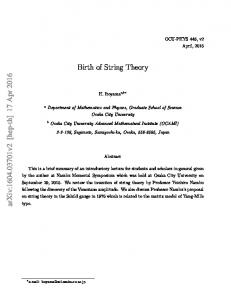
(3.23) Contrast this to the case of field theory, where the right hand side would be zero, giving us the light-cone. This is as expected for point-like behaviour. The flat space string theory result gives us a hyperbola. This is the manifestation of the halo which broadens out the available region of contact by widening the light-cone into a sort of "light-funnel". For the f-L =/= 0 case, the hyperbola is deformed, since z- decreases more rapidly with increasing z+ than before due to the behaviour of the function D(f-Lz+) discussed below equation (3.19). See figure 3.2.

z

,. / / / /

/

'

/

/ / /

z

Figure 3.2: The hyperbola (solid curve) represents the edge of the "halo" for D-instantons in flat space, p, = 0. For the f-L =f 0 case, it is deformed to the dashed curve. The field theory result is the pair of lines z+ z- = 0. For the interpretation of the shape of the halo for non-zero f-L once the transverse positions of the branes are different from each other, more work is needed. This is because the metric is no longer fiat, and furthermore, we have to take seriously the matter of the Euclidean continuation of the metric implied in the computation of the amplitude. The choices made mean that the metric is no longer real (see equa-

3. 3. Summary

36

tion (3. 21)), and this presents difficulties of interpretation which must be explored further.

3.3

Summary

We have seen that the structure of the halo for Lorentzian branes in the plane wave background is independent of f-L, giving the same physics as for D-branes in fiat space. This is because the mass parameter induced by non-zero f-L in the effective world-volume theory vanishes in the open string IR limit, the regime where the halo is to be found. For the D-instanton (and presumably all Euclidean branes) this is not the case, since their being pointlike in the x± directions requires the relevant amplitudes to be defined by starting with the closed string light cone gauge and then arriving at the open string physics by duality. The resulting open string physics sees a mass parameter which does not vanish in the IR limit, and hence the physics of the halo is not the same as in fiat space. The significance of this non-trivial 1-L dependence of the structure of the halo of the D-instanton (and by extension, all Euclidean branes defined by starting with the closed string amplitude) is not clear at present. However, it may have some significance, since D-instantons contribute to type liB string theory processes non-perturbatively (see e.g., ref. [60]). See also ref. [61] for another study of D-brane interactions in plane wave backgrounds where the difference in Euclidean and Lorentzian branes is discussed.

Chapter 4

T.,.dualities in null directions, and closed timelike curves This chapter is a detour from the general theme of exact string theory solutions, but nevertheless serves as a motivational link between the study of plane waves in previous chapters, and the study of stringy Taub-NUT spacetime in the next chapters. The central issues are T-dualities in null/timelike directions and closed timelike curves, which I will address by studying a rotating Dl-D5-pp supergravity solution. We saw in section 2.4 that the Hagedorn temperature of thermal string theory is related to the self-dual radius under a T-duality transformation. And in order to carry this correspondence on to the plane wave solution, we were led to consider T-dualities in null or timelike directions. In this chapter I pick up this question, but in a more general context. The spacetime we will study has a parameter J (angular momentum) which may serve as a regulator, allowing investigation ofT-dualities that may become null or timelike in a controlled way. I will first introduce the particular supergravity solution, and then consider various T-duals of it. Next, I will investigate probes in the resulting solutions, and finally discuss the issue of closed timelike curves in these spacetimes.

4.1

Introduction

The model I will consider in this chapter is the type IIb supergravity solution corresponding to a rotating Dl-D5-pp system [62]. This is a bound system of Dland D5-branes with pp-wave (parallel plane wave) excitation in one direction, and with an angular momentum (rotation). It is a 10-dimensional uplift of the arbitrary charge generalisation [63] of the 5-dimensional BMPV black hole solution [64]. The

37

4.1. Introduction

38

bosonic fields of the supergravity solution are [62] (the below form of the RR-fields was given in ref. [65]):

(4.lb)

(4.lc)

where the harmonic functions H 1 , H 5 and Hp are given by (4.2) and M is a four-dimensional manifold which can be T 4 or K3. The asymptotic volume of M is denoted V, and ds'it is the unit volume element on M. The zdirection is a circle of length 21r Rz, and the angular coordinates take values according to 0 E [0, ~], cP1 E [0, 27r), c/>2 E [0, 27r). The parameter J is the angular momentum, while the parameters r 1 and r 5 quantify the Dl- and D5-brane charges, and rp quantifies the pp-wave charge. The antisymmetric B-field vanishes in this solution. The metric has a horizon at r = 0, and the part of spacetime within the horizon is not accessible in these coordinates. In order to check that the solution is consistent with the supergravity equations of motion, it is necessary to Hodge-dualise the 6-form C( 6 ) to get a 2-form, and then add it to the other 2-form. That is, write dC( 2 ) = dC( 2 ) + *dC(6 ), which gives

C( 2)

=

H1 1 dt 1\ dz + r~ cos 2 Bd¢ 1 1\ d¢ 2 + H1 1 J 3 r(sin 2 Bd¢ 1 - cos 2 Bd¢ 2 ) 2r

1\ (dz- dt).

(4.3)

Because it will ease the notation later on, let me define the three functions T, S

4.1. Introduction

39

and U by (4.4) (4.5)

(4.6) Before proceeding, it is worth making some observation about the properties of this solution. First, consider the Killing vector (4.7)

with a length

for the chosen function a. (The a was chosen to make the last term in the above expression vanish, i.e. to give a "maximally timelike" vector. ) Define

(4.9) If J > J* we can have T(r)

< 0, and the vector f is a timelike Killing vector for

r < rch(J), where rch(J) is defined by the equation T(rch) = 0. Since z is a compact direction, the vector f can be the tangent of a closed curve. And it being timelike therefore means there are closed timelike curves (CTCs). For this reason the radius rch ( J) is referred to as the chronology horizon. Solutions with J < J* are called under-rotating, while those with J > J* are called over-rotating. I will return to the issue of closed timelike curves in section 4.4. Another observation concerns the 5-dimensional spacetime resulting from a KaluzaKlein reduction on M and on z. This spacetime is the three-charge generalisation of the BMPV black hole. The entropy of this black hole, as usual given by the area of the horizon, is (62]:

(4.10) where G 5 is the 5-dimensional Newton's constant. The entropy becomes imaginary in the over-rotating case, J > J*.

40

4.2. T-dualities

4.2

T-dualities

As I will come back to again later, the rotating D1-D5-pp solution and its T-duals have compact directions which become timelike if the rotation J is above the critical value J*. This is interesting, since we can view the parameter J as a regulator, allowing us a window into the physics ofT-duality along a null direction. After one T-duality transformation the potentially timelike compact direction is a coordinate isometry direction, making possible a particularly simple approach to the study of T -duality along a null direction. The idea is therefore to do a second T-duality along this potentially timelike direction, assuming it is spacelike (i.e.,. assuming J < J*). Then, at the end, we can investigate the limit where J tends to, or become greater than J*. Taking this limit on the component fields will lead to divergences, but it is nevertheless possible that appropriate probes will see a non-singular spacetime. Such probe calculations will be carried out in section 4.3. Now, let us focus on T-duality transformations. A T-duality transformation along some coordinate direction

x gives the dual NSNS fields

(denoted with a tilde)

[66,67]: -

1

Gxx=a,

XX

(4.11)

where the index i takes values for all directions except X· The dual RR potentials are [68]: C(n)_

= C~n-:-1) _

t ...Jkx

c 1 z-dual solution forward calculations reveal that det P(9ab) = det 9ab

+ 2(9zz9tm - 9tz9zm)X· m + (9zz9mn - 9mz9nz)X· m X·n + O(X· 3 ) ,

det 9ab = - (H1H5) 2 s- 2 . ( 4.18)

In the slow motion approximation the square root can be expanded, leading to

( 4.19)

where vi = xi, and i, j now run over all transverse directions except r and ¢ 2 . The induced B-field has only one component P(B)tz which becomes

P(B)tz = BJ.LIIOtX1Lf3zX 11 = Btz + Bmzj(m = -1

_1

+ (H1H5)S - (H1H5)S

_1

(4.20)

J cos2 B · r2

2

0 we only have T > 0. That is, we only get spacelike geodesics. The same holds for case (ii). Case (iii) leads to the equation (4.41)

which is never satisfied (the left hand side is always positive). So, again, we find no CTCs which are geodesics. An interesting question to ask is whether the CTCs not being geodesics is aTduality invariant statement. These calculations suggest so, and also those of ref. [80]. But these examples are of course not enough to state this as a general fact, and it would be very interesting to study this further.

4. 5

Discussion

Timelike T-dualities have been studied in refs. [83, 84], and was shown to relate type Ila (lib) string theories to so-called type lib* (II a*) string theories.

The

type II* supergravities are similar to type II, except for sign differences. These are nonetheless important differences, and imply that type II* supergravities have ghosts. In the gravity/ gauge duality picture, they correspond to non-unitary gauge theories also with ghosts. However, these ghosts are believed to be an artefact of the supergravity truncation, and the full type II* string theories are supposed to be ghost-free. We have seen that the the existence of closed timelike curves is not affected by the T-dualities, which supports intuition based on the fact that a T-duality transformation does not change the physics.

As long as we stay in the under-

rotating regime J < J* the T-dual solutions are not very exotic - they share the same properties as the original solutions, but are just more complicated. If we

4.5. Discussion

53

approach the over-rotating regime J > J*, we have seen that there are divergences appearing in the components of the T,hz-dual solution that are associated with a Tduality transformation being taken along a null direction. This is an expected result, as it follows immediately from the transformation rules (4.11). A more interesting result is the fact that various probes put into this spacetime are free of the same divergence. A possible interpretation of this is that the divergence is an artefact of the supergravity truncation that is somehow resolved by properly taking into account o/ corrections incorporated in the probes. Essentially, we ought to remember that the elementary objects in the geometry are not points as assumed in the supergravity approximation, but extended strings and branes. Furthermore, the result suggests that T-duality transformations in null or even timelike directions make sense with the same corrections taken into account. We have also seen that none of the CTCs satisfy the geodesic equation, and are therefore not geodesics. However, this does not necessarily mean that no CTCs can be geodesics, since there might be other CTCs in these spacetimes than those I have discussed. A general investigation of the geodesic by a Lagrangian approach would make the answer definite. But in these spacetimes, with so few symmetries, such a study is highly non-trivial. The problem of closed timelike curves is one of the prime motivations for the work of the remaining part of this thesis. In chapter 6 I will describe an exact model where it is possible to compute all a' corrections to the supergravity solution, and see how those change the discussion of CTCs.

Before going into details on

that, however, a more general discussion of Wess-Zumino-Witten-Novikov models is necessary.

Chapter 5

Wess=Zumino=Novikov= Witten models In the previous chapter we saw the existence of closed timelike curves in a solution to supergravity, but did not dwell on the significance or interpretation of such curves. One immediate question that comes to mind is how full string theory might modify this picture: Will the problems associated with closed timelike curves be resolved in string theory beyond the supergravity limit? For the remaining part of this thesis I will study an exact string theory model (and a generalisation of it) where this question can be addressed properly and to some extent answered by direct calculations. But before turning to the particular models, I will in this chapter present the necessary concepts and techniques that are the basis for the next two chapters. First, I will introduce the Wess-ZuminoNovikov-Witten model in section 5.1, and how it is related to coset constructions in two-dimensional conformal field theory in section 5.2. Section 5.3 is a presentation of a method for extracting the exact spacetime fields from coset models. Then in section 5.4 I discuss heterotic coset models, which are the type of constructions we will use in the subsequent chapters. Section 5.5 gives an example of how the ideas are applied in the case of a two-dimensional charged black hole.

5.1

WZNW models

Wess-Zumino-Novikov-Witten (WZNW) models (85-87) are conformal field theories (CFTs) in which a current algebra gives the spectrum of the theory. They can be given a Lagrangian formulation as nonlinear sigma models on a group manifold with an antisymmetric tensor background, and provide a very useful setting in which to study many aspects of string theory, as is apparent from the large amount of 54

5.1. WZNW models

55

attention such models have attracted. In string theory, these models correspond to bosonic strings propagating on a group manifold. An introduction to WZNW models can be found in ref. [88]. Such models were first studied in the context of two-dimensional bosonisation, giving the bosonisation rules for non-interacting massless fermions [85].

It was

demonstrated that a theory with N massless free Majorana fermions is equivalent to a theory with N massless free bosons with global symmetry O(N), which can be expressed as a WZNW model based on the group O(N). Current algebras

Consider a general CFT with a set of (1, 0) currents ja(z). If

we expand the currents as a Laurent series, ·a ( )

J

Z

=

"'"""' ·a

6JmZ

-m-1

(5.1)

'

m

then the conformal invariance implies that the modes satisfy the following algebra ·a Jn ·b] [Jm,

·c = 't·jabcJm+n + ffi kdab!;Um+n·

(5.2)

Note that (j0, jg] = irbcj0, so rbc are the structure constants of the Lie algebra satisfied by the zero modes. The term proportional to k is a central extension, often referred to as a Schwinger term. The factor dab is the Lie algebra inner derivative, defined as dab= (Ta, Tb), with {Ta} being a basis for the algebra. The constant k is the level constant. The algebra (5.2) is known as a current algebra, or affine Lie algebra, or affine Kac-Moody algebra. It is common to denote this algebra

Gk,

where Go= Lie(G) is

the associated Lie algebra corresponding to a Lie group G. \Ne can study the current algebra and find out lots of things about the theory.

Particularly useful is the so-called Sugawara construction which gives the energymomentum tensor as a product of two currents. Essentially, it says that the Virasoro algebra belongs to the enveloping algebra of the current algebra. The exact connection between the energy-momentum tensor and the currents is a remarkable feature of current algebras with conformal symmetry in two dimensions. I will not go into any more detail on this, but refer to refs. [14,88,89] for thorough treatments of current algebras, and other aspects of conformal field theory. Although much can be found out by studying the current algebra, it is also very useful to have a Lagrangian formulation of the theory. And this is exactly what the WZNW models provide. Consider a Lie group G, and let g E G be a map from the

5.1. WZNW models

56

worldsheet :E to the group G, g : :E

where

r(g)

-----t

G. Then the \VZNW action is

1

= - -

( Tr(g- 1 dg) 3

(5.4)

121f}B

is known as a Wess-Zumino term. The constant k is the same as the level constant in the current algebra (5.2). I have used the notation 8 = 02 ,

8 = 82 . :E

is the

embedding of the worldsheet in the group manifold G, and B is a three-dimensional surface whose boundary is :E. The Wess-Zumino term is a three-dimensional integral, but since the integrand can be written as a total derivative it can locally (albeit not globally) be rewritten as an integral over the worldsheet :E. To see explicitly that the WZNW action can be written as a standard nonlinear sigma model, we should parameterise the group element as g = eiTJlXJJ., where Tf..L are generators of the group. The WZNW action then becomes I=

= =

.!5_ ( d2zTr(TJ.LTv)8XIl[}Xv + - 1- ( Tr(TJ.LTvTp)dXf..L 1\ dXv 1\ dXP 47r }y:, 127r } B

4~ 1d zTr(TJ.LTv)8XIl[}Xv + 1 ~7r fa d aTr(Tf..LTvTp)cabc8aXf..Lf}bXv8cXP 4~ 1d z(Tr(TJ.LTv) + Tr(Trf..LTv]Tp)c XP )oxJ.L[)Xv. 2

3

(5.5)

22

2

This is of the form of the nonlinear sigma model

(5.6) with the metric GJ.Lv = Tr(Tf..LTv), and antisymmetric B-field BJ.Lv = Tr(T[J.LTv]Tp)XP. The level constant k should be identified with the string tension, k "' 1,. So the a low-energy regime a/

-----t

0 corresponds to k

-----t

oo.

Despite this connection, there is one property of the WZNW models not shared in general by nonlinear sigma models that makes them particularly interesting. Namely the fact that they are described by an exact CFT. Nonlinear sigma models are string theories formulated in a particular background, and valid to first order in a'. On the other hand, WZNW models, through the CFT description, are well defined independently of any background spacetime. It has a purely worldsheet formulation valid for any value of a/.

5.2. Coset models as gauged WZNW models

5.2

57

Coset models as gauged WZNW models

Coset models were invented [90, 91] in the early seventies, and later generalised [92, 93] as algebraic realisations of new conformal systems GI H based upon current algebras for a group G and a subgroup H. An important property of CFTs with current algebra is that they can always be factored into two completely independent parts [14]: One Sugaware part and one part that commutes with the current algebra. That is, the CFT splits into a Sugawara theory, with an energy-momentum tensor T 8 obtained via the Sugawara construction entirely from the current, and another CFT with an energy-momentum tensor T' that commutes with the current. The total energy-momentum tensor can then be written T =

rs + T'.

G and a subalgebra fi C G, this means that we energy-momentum tensor T 6 = Tii + T 6 1ii. For any subalgebra,

In the case of a current algebra can split up the

the Sugawara theory separates into the Sugawara theory of the subalgebra, and a new coset CFT. A representation Xr of the

G current

algebra can be decomposed under the

subalgebra, c _ "" r ii c;ii Xr - L...t nr'r" Xr' Xr" ,

(5.7)

r',r''

where r' and r" runs over all representations of ii and GIii respectively, and n;'r" are non-zero integers. Since current algebra theories are quite well understood, this is often a very useful way to represent the coset theory. Within the Lagrangian formulation, the coset construction can be regarded as a gauging of the subalgebra H. Conformal invariance forbids a kinetic term for the gauge field, and the equations of motion for this field then requires the H -charge to vanish, leaving only the coset theory. The coupling to the gauge fields A is straightforward for the metric part of the WZNW action. We simply use minimal coupling, and replace derivatives with covariant derivatives, roughly

a

-t

D =

a + A.

The metric part is then gauge

invariant by itself. The Wess-Zumino term f(g), on the other hand, poses some difficulty. It does not allow a gauge invariant extension for general subgroup H. However, there is a unique extension which is such that its variation under a gauge transformation only depends on the gauge fields and not on the group element g E G [94]. Assume that the ungauged model has the symmetry group G L x GR, where the subscripts L and R denote left and right action respectively. This means that the

5.2. Coset models as gauged WZNW models

58

action is invariant under the global transformation

g(z, z) --+ [h g(z, z) 9"R 1 ,

(5.8)

We want to promote this to a local symmetry. In other words, we want the action to be invariant under local transformation in a subgroup H

c

G, i.e., we impose

the symmetry (5.9)

In the special case that h"R 1

= hL,

this is called an axial gauging, and if hR

= hL

it

is called a vector gauging. To realise this symmetry, introduce the gauge fields A~ and the covariant derivative (5.10)

where Tl,Tk (i = 1, ... , dim(H)) are generators of the subgroup H, and I am using the notationAL= A~T{daa = AL,adCJa and AR = A~Tkdaa = AR,adCJa. The unique extension [94] of the Wess-Zumino term is then

r(g)--+ f(g)

+ 4~

J[A~daa

A Tr(Tldgg-

1

+ Tkg- 1 dg)

1 1 + ~Ai Aidaa A dabTr(TigTigTigTig)] 2ab R L R L ·

(5.11)

Putting this together, the action for the gauged WZNW model [95-100] becomes 1

(5.12)

Since there is no gauge-invariant extension for the Wess-Zumino term f(g) for general subgroup H, this action has (in general) classical anomalies. Only certain subgroups and gaugings therefore give sensible theories, singled out by the condition of anomaly cancellation. Consider the gauge variation oA~ = Baai, og = ai(T{g- gTk). This leads to the Expressions in the literature often differ from this one by the interchange z f--7 z, which amounts to subtracting rather than adding the extension to r (g)' or to define fzz = + 1 rather than -1. 1

5. 3. Exact spacetime fields from coset models

59

anomaly (5.13)

So the anomaly cancellation condition is (5.14)

By using gauged WZNW models, actions can be written for a large class of conformal field theories obtained as coset models. Let me briefly recapitulate: The ungauged model has some global symmetry group G which defines a conformal field theory [101-103] with an underlying current algebra. Coupling it to gauge fields charged under a subgroup H C G gives the coset, as reviewed above. Such models have been used to generate conformal field theories for many studies in string theory, including cosmological contexts. It is important to note that the vast majority of these models use a particular sort of gauging. The basic worldsheet field g(z, z) is group valued, and the full global invariance is GL x GR, realised as: g(z,z)-+ gLg(z,z)g"F/, for 9L,9R E G. The sorts of group

actions gauged in most studies are g

-+

hLgh]/, for hL, hR E H, and it is only a

restricted set of choices of the action of hL and hR which allows for the writing of a gauge invariant action. These are the "anomaly-free" subgroups, and the typical choice that is made is to correlate the left and right actions so that the choice is essentially left-right symmetric (axial or vector gauging). This also gives a symmetric structure on the worldsheet, as appropriate to bosonic strings and to superstrings if one considers supersymmetric WZNW models. For these anomaly-free subgroups, a gauge extension of the basic WZNW action can be written which isH-invariant, and the resulting conformal field theory is well-defined. The supersymmetric models can of course be turned into heterotic string theories too, by simply tensoring with the remaining conformal field theory structures needed to make a left-right asymmetric model. I will return to heterotic models in section 5.4.

5. 3

Exact spacetime fields from coset models

In this section I will review the procedure for extracting the exact spacetime fields from the gauged WZNW model. The idea [104] is very simple: Integrate out the gauge fields, compare the resulting action to the nonlinear sigma model, and read off the fields. However, if we do this directly, the result is only going to be valid to first order in the parameter k, since the procedure of integrating out the gauge fields in the naive way is only valid

5.3. Exact spacetime fields from coset models

60

to first order. The reason for this is that we are treating the gauge fields as classical fields, substituting their on-shell behaviour into the action to derive the effective nonlinear sigma model action for the rest of the fields, and ignoring the effects of quantum fluctuations arising at subleading order in the large k expansion. To include all of the physics and derive a result valid at any order in k, we need to do better than this. This sort of thing has been achieved before, using a number of methods. The first time in ref. [105] in the context of the SL(2, IR)/U(1) coset model studied as a model of a two-dimensional black hole [104]. (See also section 5.3.4.) The exact metric and dilaton were deduced by appealing to a group theoretic argument, writing the exact expressions for the quadratic Casimirs for

G and for H, in terms of the target space (G /H) fields, and then equating their difference to the Laplacian for the propagation of a massless field (the tachyon) in the background. The proposed metric and dilaton were verified at higher orders by explicit calculation in refs. [106, 107], and the argument was generalised and applied to a number of other models in a series of papers [108, 109]. An elegant alternative method was developed in refs. [110, 111], and is the one I will adapt for use in the following. The basic idea of this method is to first deduce a quantum effective action which takes into account the higher energy modifications of the classical action, and then integrate out the gauge fields. Since the effective action already encodes high energy effects, this integration can be done accurately by simply solving the equations of motion and substituting back. Done this way, the fields we read off will be valid to all orders in k.

5.3.1

The Exact Effective Action

The first thing to do is therefore to write down the effective action, which in general is not a simple task. But it is known [110, 112, 113] that the exact effective action for the ungauged WZNW model defined in eq. (5.3) is extremely simple to write down: Take the form of the basic action at level k, k!(g), where g EGis a quantum field, and write for the full quantum effective action (k- cc)I(g), where now g should be taken as a classical field, and cc is the dual Coxeter number of the group G. This is particularly simple since k only enters the action as an overall multiplicative factor, which then gets shifted, i.e.,

klwzNw(g)

--+

(5.15)

(k- cc)IwzNw(g).

The key observation of refs. [110, 111] is that this can be applied to a gauged WZNW model as well, by exploiting the fact that if we write Az

=

8zhzh; 1 and

5. 3. Exact spacetime fields from coset models

61

A 2 = 8 2 h 2 hi_ 1 , the action can be written as the sum of two formally decoupled

WZNW models, one for the field 9' = hi_ 1 9hz at level k and the other for the field h'

=

hi_ 1 hz at level 2cH - k. To write the exact effective action, shift the levels in

each action: k

---+

k- cc and 2cH - k

---+

2cH - k- cH

= cH - k, and treat the fields

as classical. Transforming back to the original variables, we get the original gauged WZNW model with its level shifted according to k

---+

k- cc, together with a set of

new terms for Az, A 2 which are proportional to cH- cc, and have no k dependence. Because there is no multiplicative factor of k in these new terms, it is easy to see that the large k contribution to the result of integrating out the gauge fields will be the same as as if we had used the classical action. For results exact in k, there will be a family of new contributions to the nonlinear sigma model couplings upon integrating out the gauge fields. In this effective action, they are to be treated as classical fields now and so once the integration is done, there are no further contributions from quantum fluctuations to take into account. The metrics derived using this method are the same as those constructed using the algebraic approach, which is a useful consistency check [110, 111]. Note that the new pieces in the effective action are non-local in the fields Az, A 2 (although local in the hz, h 2 ). This difficulty does not present a problem for the purposes of reading off the spacetime fields, since it is enough to work in the zeromode sector of the string to capture this information. This amounts to dropping all derivatives with respect to

O"

on the world-sheet and working with the reduced

"point-particle" Lagrangian for that aspect of the computation [111].

5.3.2

Computation of the Exact Effective Action

Let us assume that the complete classical action is a GI H = G 1 x · · · x G NIH gauged WZNW action. A group element 9 E G can then be split up

0

0

0 92

0

0

0

0

0

0

9N

91

9=

(5.16)

and the action becomes a sum of WZNW actions (5.17) m

with 9m E Gm.

62

5.3. Exact spacetime fields from coset models

We are going to gauge a subgroup H C G, and so we introduce the covariant derivative as defined in eq.(5.10). The connections take values in the Lie algebra of H. The

A~

are the gauge fields, which

Ti,L are left generators, and

Ti,R

are right

generators of H. Using the block diagonal notation above, we can write

O ) E Lie(H).

(5.18)

T.(N) l

The gauged WZNW model (5.12) is then also a sum of terms corresponding to each factor Gm in the group G, (5.19) m

where

sl (g, A)

=

4~

J zTr{ d2

A:z,LOzgg-] - Az,Rg- 18:zg- A:z,LgAz,Rg- 1

+ ~(Az LAz L + Az RAz R)} 2 !

I

l

(5.20)

·

I

The anomaly cancellation condition (5.14) generalises to (5.21) m,i

A Change of variables By the change of variables

h,h

E

H,

(5.22)

we find

S1(g, h)=

4~

J zTr{d2

Ozgg- 18:zh:zh-; 1 + g- 1 8:zg8)~,zh-; 1

- O:zh 2 h-; 1g8zhzh-; 1g- 1

+ ~(82 h 2 h-; 1 ozhzh-; 1 + 82 h 2 h-; 18zhzh-; 1 )}

.

(5.23)

5. 3. Exact spacetime fields from coset models

63

The Polyakov-Wiegmann identity [86, 114] implies:

4 j d zTr [-azhzh;- azgg-

+ ~

I(h;- 1 hz) =l(h;- 1 )

- 1-

-

I(h; hz) =l(h;- 1 )

2

1

4

+ I(hz) + ~

- + 27r + I(hz) 4

J J2

1

-

azhzh;- 1 ga)1zh:; 1g- 1 + g- 1 a2 ga)i)i_;- 1J

d2zTr [-azhzh;- 1 azhzh_;- 1 J ,

[ - - 1 - - 1]

d zTr -azhzh; Ozhzh_;

(5.24)

Using these, the classical action (5.19) can be written as

S 1 = - I(g) where

-1-] 1] , + I(h; 1ghz)- '1[ 2 I(h; 1hz) + I(h; hz) - 2C C

= I(h;- 1 ) - I(h;- 1 ) - I(hz) + I(hz)

.

The term C is not manifestly gauge invariant, but the others are. Note that if AL

=

AR, then C = 0, in which case the gauging is classically anomaly-free. Otherwise,

the anomalous terms

2:. k(i)Ci =

Ci

may look disturbing, but in fact they cancel in the action,

0, as follows from the condition of anomaly cancellation (5.21).

The change of variables (5.22) gives rise to a Jacobian which can be re-written as an additional term in the action, proportional to the dual Coxeter number

cH

of

the subgroup 2 , (5.25) Taking all this into account, and assuming we have chosen a gauging which is overall non-anomalous, we can write the action as: (5.26) Note that hi 1 ghz E G, hi 1 hz E H, and hi 1 hz E H. As promised in the previous section we have achieved to rewrite of the full action in the form of a sum of ungauged WZNW actions, which allows us to write down the quantum effective action in a very simple way. 2

1 will later only consider cases where the dual Coxeter number is zero, in which cases this Jacobian vanishes.

,

64

5. 3. Exact spacetime fields from coset models

Effective action Using the simple prescription given above, for

G: k(i) -+ k(i) -

for H: -

k(i)

+ 2cH

cci , -+ ( -k(i)

+ 2cH) -

cH

=

(5.27) -(k(i) - cH) ,

we find the effective action

(5.28)

Again, the action is manifestly gauge invariant.

Return to the original variables We now change variables back to the original ones, using the identities given above. The result is seff

=-

L {(k(i)- ccJ [I(g) + SI(g, A)+~ [I2(AL) + 12(AR)] + ~ci] i

where I2(AL)

(5.29)

=

I(hi 1 hz), 12 (AR) _ I(h-; 1 hz)· Observe that the Ci's have come

back into the action (in a combination that does not cancel). Rewritten, this is seff

=-

L(k(i)-

ccJ [I(g)

+ SI(g, A)- ~i [I2(AL) + 12(AR)]]

'

(5.30)

i

, ca.-cH where "'i = k (i)-CG; . Since we consider the fields in the effective action to be classical, there is no Jacobian associated with this change of variables.

5.3.3

Extracting the Exact Geometry

As stated earlier, a problem with working with this action is that it has terms which are non-local in the gauge fields. Since we are going to integrate these out, this is inconvenient. To avoid this complication, we reduce to the zero mode sector [111), which is enough to extract the information we want.

The zero mode sector is

obtained by letting fields depend on worldsheet time only. So replaced by

aT.

az and 8-z are both

We also denote A by a in this limit. This leads to the desired

5. 3. Exact spacetime fields from coset models

65

simplifications. An additional simplification is that the WZ part f(g) of the WZNW action vanishes in this sector. The resulting action is

sgff = -

JdT{

L (k(i) 4~ ccJ

Tr(g-logg-log)

t

+ 2Tr[a.z,LOgg- 1 -

1

az,R9- 10g- az,L9az,R9- 1 + 2(az,Laz,L

+ az,Raz,R)]

Ai~Tr[(az,L- az,L) 2 + (az,R- az,R) 2 ]

+ ~ Tr [az,Raz,R - az,Raz,R + az,Laz,L - az,Laz,L] } . (5.31)

This is a local action quadratic in a. It is useful to simplify the notation, so let me define

La= L'tJEJXM

=

L(k(i)- ccJTr(TR,a9- 1 8g) , i

-Ra

=

-R'tJoXM =

I)k(i)- ccJTr(TL,aogg- 1 )

,

i

Mab = L(k(i) - ccJTr(TL,a9TR,b9-l- TL,aTL,b) , i

Mab = L(k(i) - ccJTr(TL,b9TR,a9-l- TR,aTR,b) = Mba+ 2Hab , i

1

Gab= L(k(i) - ccJ>-i2Tr(TL,aTL,b + TR,aTR,b) i

1

z:)cci- cH)2Tr(TL,aTL,b + TR,aTR,b)'

=

i

Hab

1

=

2:)k(i)- ccJ2Tr(TL,aTL,b- TR,aTR,b)

'

i

(5.32)

In this notation the action can be written as:

Sgff = - ~

4

JdT{

g-

-

2a~Ra- 2a~La- 2a~a~(Mab- Gab+ Hab)

a~a~(Gab + Hab)- a~a~(Gab- Hab)} .

(5.33)

5. 3. Exact spacetime fields from coset models

66

Defining

Aij

where G+ = G form

+H

=

G_ M- G_) ( ) ( M- G+ G+ , 5.34 ~

and G_ = G- H, the action can be written in the compact Sgff = -

4~ JdT{ g- 2Bizi- ziAijZj} .

(5.35)

Now we complete the square, and get (5.36) where

Akl

= (A- 1 )k1.

The equations of motion for z (i.e., the equations of motion for the gauge fields

az and a2 ) are easily read off, (5.37) Inserting this into the action, we arrive at (5.38) To write out this explicitly, we need to invert the matrix Aij. If we write this inverted matrix as (5.39) then equation (5.37) gives a~ = -PabRb - qabLb ,

(5.40)

a~

(5.41)

= -rabRb

-

SabLb '

and

(5.42)

5. 3. Exact spacetime fields from coset models

67

This action is of the form of the nonlinear sigma-model, and we can extract the exact spacetime fields from the coefficients C M N. Furthermore, finding the coefficients

CMN

means finding the matrices

p, q,

r, s.

Explicitly, (5.43)

where I have included the antisymmetric field bMN which is the counterpart to gMN, and comes from the WZ term. Its contribution vanishes here in the zero mode sector, but it will be relevant for reading off the B-field. Note that with this definition,

CMN

is not automatically symmetric. The metric is now easily read off by symmetrising CM N, cMN

=

c(MN)·

(5.44)

The dilaton is a one-loop effect which is given by a determinant coming from the integration of the gauge fields, (5.45)

To get the B-field really requires going beyond the zero-mode sector. But there is a trick to do this without any extra work [111 J. Simply take advantage of the fact that the local part of the action is (5.46)

so that the B-field is given by antisymmetrising

CMN,

(5.47)

Thus we have found general expressions for the exact (in a') spacetime fields

G M N, B M N and for coset models.

5.3.4

Example: A 2D black hole

As a simple example of how this works, let us now consider the two-dimensional black hole spacetime [104] corresponding to the coset SL(2, lR)/U(l). The exact metric and dilaton were first worked out in ref. [105] using a Hamiltonian approach. The computation has been done over again in ref. (110] using roughly the same

5. 3. Exact spacetime fields from coset models

68

method as presented here. Start by parameterising the group element g, and the gauge symmetry generators

TL, TR according to e t:+

sinh~

) E SL(2, IR),

e-2 cosh~

(5.48) (5.49)

where t± = tL ± tR. This gauging is an axial gauging, g---+ eT ger, and is classically non-anomalous, which means the anomaly cancellation condition is automatically satisfied. For this coset we have cc = 2, cH = 0, ,\ = k~ 2 . Let us also choose unitary gauge where tL = 0 (giving t+ = tR, We then find H = 0,

= -tR)·

t_

2),\~,

G = (k- 2).\Tr(TT) = (k-

(5.50)

and furthermore

gp.v()XP.()Xv = (k.M

2)~(d0" 2 + dt~),

= M = (k- 2)Tr(TgTg- 1 - TT) = (k- 2)(cosh 2 ~- 1), (5.51)

1

Lp.()XP. = (k- 2)Tr(Tg- 18g) = (k- 2)(28tR), Rp.()XP.

=

1

(k- 2)Tr(T8gg- ) = (k- 2)(cosh

1 '2- '2)8tR,

2 (}

and p - s - -

-

-

G

,\

- ~-----------;;-----~ M(A1-2G)- (k-2)2sinh 2 ~(-cosh 2 ~+1+,\)'

M - G -2 cosh ~ + 2 + ,\ q - r - ~---:-----;c;----:-=---;;----~ - M(M- 2G) - (k- 2)2 sinh 2 ~(- cosh 2 ~ + 1 + ,\)' 2

(5.52)

This gives the exact metric dS 2

_ -

k - 2 [ (cosh O" + 1 2 coshO"- 1

-- -

-

2 ) - 1 dtR2 k

-

+ d0" 2]

(5.53)

together with a vanishing B-field, and the dilaton (5.54)

5.4. Heterotic coset models

5.4

69

Heterotic coset models

The heterotic coset model technique which I will describe in this section, was introduced in ref. [115] as a way to study more general coset models. It goes beyond the coset construction as described in section 5.2, and exploits the basic fact that the heterotic string is asymmetric in how it is built. The idea is to allow ourselves the freedom to choose to gauge far more general subgroups. This might well produce anomalies, but permits us to choose to keep certain global symmetries which might be of interest (such as spacetime rotations) and/ or use in the conformal field theory. Introducing right-moving fermions to achieve a right-moving supersymmetry is easy to do, and they contribute extra terms to the anomaly, making matters worse in general: Their couplings (the effective charges they carry under H) are completely determined by supersymmetry, so we have no choice. Of course, we do not have a well-defined model if there are anomalies, so ultimately they must be eliminated. This is achieved as follows [115]. Note that the left-moving fermions can be introduced with arbitrary couplings (charges under H), since there is no requirement of left-moving supersymmetry in the heterotic string. The anomaly they contribute comes with the opposite sign to that of the others, since they have the opposite chirality. The requirement that the anomaly cancels can be satisfied, since it just gives a set of algebraic equations to solve for the charges. The resulting model is a conformal field theory with (0,1) worldsheet supersymmetry, (enhanced to (0, 2) when G / H is Kahler [116-118]) naturally adapted to the heterotic string. It is important to note that the types of heterotic models obtained by this method

are very different from the types of models obtained by gaugings that do not cancel the anomalies against those of the gauge fermions. One way to see the difference is to note that since the anomaly is proportional to k, the cancellation equation puts the gauge charge at the same order as the metric. This means that there is a nontrivial modification of the geometry that we would read off from the WZNW action, traceable to the left-moving fermions. We will see this in detail in the following. The method described in the previous section for extracting the exact spacetime fields in coset models has to be extended to work for heterotic coset models. Although heterotic backgrounds have been considered in some previous works [108], they are of the mildly heterotic type which are essentially similar to the superstring models: an asymmetric arrangement of fermions is merely tensored in as dressing. The crucial fact that makes the same ideas work also with fermions included, is that the fermions, through non-Abelian bosonisation, can also be written as a gauged WZNW model. The issue of non-Abelian bosonisation was in fact what historically led to the WZNW model in the first place [85].

70

5.4. Heterotic coset models

5.4.1

Abelian bosonisation

The technique of bosonisation is based on the remarkable equivalence in two dimensions between theories of fermions and theories of bosons. The simplest example of this is the equivalence between massless free Dirac fermions and massless free scalar bosons. Before turning to non-Abelian bosonisation, which is really what I am interested in, let me first summarise the basic Abelian bosonisation rules. In terms of a Dirac spinor W and a real boson .AV2 AA + ~FP"!.B >,A >.B,(fp-J;a J (5.69)

where the covariant derivatives are

(5. 70) (5.71)

The A's and 'lj;'s are the left- and right-moving fermions respectively, and F and Hta are the field strengths corresponding to the gauge potential AJl. and antisymmetric tensor potential BJl.v respectively. The quantity

r~a

is the spin connection, associated

with the metric GJ.Lv· When reading off the spacetime fields from our heterotic coset model, this is the action we have to compare to. But there is a small problem, since we have the action presented in a fully bosonised form. The idea is therefore to compare our bosonic action (expressed in a suitable form) with a bosonised version of the nonlinear sigma model. We have seen that the local part of the action can be written (where I have re-introduced dependence on worldsheet space as well as time, which is necessary to deduce the B-field) s =

where QMN

J

2

d z(QMN

+ BMN)ax M-ax N '

(5.72)

= C(MN) and BMN = G[MNJ, and the coefficients CMN are given in

eq.(5.43). Assume that the original G / H coset model is a D-dimensional model (D = dim( G)- dim(H)), and that the fermions bosonise into d bosons. Then this action as it is written is effectively a (D +d)-dimensional bosonic theory where the extra

d dimensions correspond to the bosonised fermions, i. But to deduce the correct spacetime fields, we have to take into account that the fermions really are fermions.

73

5.4. Heterotic coset models

This is therefore not the appropriate form of the action for reading off those fields. Instead, we ought to re-write it as a 4-dimensional heterotic nonlinear sigma model, and then identify the fields. In order to do that, we need to re-fermionise .Af)Tr[a3g1 18z91]- 2A~Tr[a38z9191 1 ] 2

1 +A~ A1(1 + o2 + oTr[a3g1a3gi ]) + >- 2 A~ Af + >.oA~ Af +A~ A1(>.o + >.Tr[a3g1a3g1 1])} + ::

jd

2

1

a {2iAfTr[a3g2 8z92]

+A~ A.zB}

. (6.16)

3

Actually, we can also choose other values of c, and adjust the internal theory appropriately.

89

6. 3. Exact Conformal Field Theory

The gauge generators have been written as t(l) - -60"3 A,R2'

t(l)

-

A,L-

0"3

t(l) B,R-

2'

->. cr3 2

(2)

>

-

t BR-

'

. 0"3

-~-

2

(6.17)

·

The anomaly under variation 6A~(B) = OaEA(B) can be written as: (6.18) (no sum on a, b) and I have defined Tr

=

-k 1 Tr 1 +k2 Tr 2 . The right-moving fermions

have an action: (6.19) where WR takes values in the orthogonal complement of the Lie algebra of U(1)A x U(1) 8 , (so there are four right-movers, in fact) and (6.20) a

The four left-moving fermions have action:

(6.21)

Under the gauge transformation 6A~(B)

=

Oaf A( B), these two sets of fermion actions

yield the anomalies discussed earlier, but at one-loop, while the WZNW model displays its anomalies classically. It is therefore difficult to work with the model in computing a number of properties. In particular, in working out the effective spacetime fields it is useful to integrate out the gauge fields. It is hard to take into account the effects of the successful anomaly cancellation if part of them are quantum and part classical. The way around this awkward state of affairs [115] is to bosonise the fermions. The anomalies of the fermions then appear as classical anomalies of the action. The bosonised action is:

Is=

4~ Jd z{ [8z 2

-sin

sin

1> 2

cos

v'2

V2

1> 2

v'2

1> 2

V2 (6.29)

where


96

6.4. Exact spacetime fields

With the above expressions for the exact spacetime fields, it is worth noting that they all diverge at D(x) = 0, and that this is the only place where they diverge. The coefficients

YMN

and

BMN,

and the dilaton before re-fermionisation had divergences

for Ll(x) = 0, so what the re-fermionisation has done is to include the back-reaction in a way which moves these to the true singularity D(x) = 0. It is highly non-trivial that this happens so nicely for all the fields.

6.4.2

Properties of the Exact Metric

As already stated in the previous section, the final result for the exact spacetime metric is (after a trivial shift in t): 2

ds 2 = (k- 2) ( 2dx X -1 F(x)

where

= -

1

x2D(x)

= -

(

+ F(x)(dt- >.cosBd¢) 2 + dB 2 + sin 2 Bd¢ 2 ) (x + 0')2 x2 -

1

_4_) k+

,

-1

2

(6.45)

This is a pleasingly simple form to result from such an involved computation. In fact, its relation to the leading order result is reminiscent in form to the relation between the leading order and exact results for the black hole SL(2,IR)/U(1) model [104,105] of section 5.3.4. It is interesting to sketch the behaviour of Gtt = F( x), as it contains the answer to

the original questions about the fate of the Taub and NUT regions of the spacetime once the contributions of the stringy physics are included. This result is plotted in· figure 6.3, and it should be contrasted with figure 6.1. Several remarks are in order.

The first is that the Taub and NUT regions,

although modified somewhat, survive to all orders. The second is that the local structure of the chronology horizons separating these regions is completely unaffected by the stringy corrections! F( x) still vanishes at x = ± 1 and furthermore for

x

=

1- T where Tis small, the metric of the (T,

of the 5

2

)

~)space

(the space over each point

becomes:

ds 2 = (k- 2) ( -(2T) -1 dT 2 +

2T0) d~ 2) (1 + 2

,

(6.46)

which is again of Misner form. Notice that the singularity we observed in F(x) (and the spacetime) has now split into two. Recalling the definition of D(x) given in equation (6.32), we can

97

6.4. Exact spacetime fields

F(x) Euclidean region

X

NUT

NUT

Figure 6.3: The various regions in the stringy Taub-NUT geometry for arbitrary k, with all 1/k corrections included. Compare to the leading order result in figure 6.1. Note that the singularity splits in order to incorporate a finite sized region of Euclidean signature in the second NUT region. write the Ricci scalar as:

R

= -

1 2 2 2 (k _ )D 2 [2D(x 2 - 1)D"- 3(x 2 - 1) (D') + >. (x - 1)D + 6xDD'] , 2 2 (6.47)

(where a prime means djdx). Note that at x

= ±1, we have a finite, non-vanishing

result for R for generic values of the parameters:

R

8(k + 2) ± (k- 2) 6 ( 2(8 + 1) 4 ) = ± 6 (1 ± 8)2(k2 - 4) = ± (8 ± 1)k 1 + k + k2 +... .

(6.48)

The curvature R diverges if and only if D(x) = 0. These singularities are located at:

-8 ± X±=

Ja

2

+ a(8 2 -

(1- a)

1)

'

4 a= k+2'

(6.49)

and the region in between them has Euclidean signature. Such a region was noticed in ref. [179] in the context of the exact metric for the SL(2, IR)/U(1) coset giving the two dimensional black hole. This region remains entirely within the second NUT region, however, and never approaches the Misner horizons. Its size goes as 1/(k-2). The model only seems to make sense for k > 2, of course, and it is interesting to

98

6. 5. Discussion note that the limiting behaviour of this metric as k

~

2+ is that the Euclidean

region grows until it fills the entire left hand side of the sketch (see figure 6.4), with one singularity at x = -(6 2

+ 1)/(26), Euclidean region

and the other one moving off to x ~ -oo.

F(x)

X

NUT

Figure 6.4: The various regions in the stringy Taub-NUT geometry for the smallest value of k possible. This is the "most stringy" geometry. Compare to the leading order result in figure 6.1 and the intermediate k result in figure 6.3. The Euclidean region has grown and occupied the entire region to the left, making the second nut region of finite extent.

6.5

Discussion

The goal in this chapter was to identify a stringy laboratory for the study of a number of issues of interest, which allows a controlled study of various physical phenomena. Closed timelike curves are very common in General Relativity, but the theory is silent about their physical role in a complete theory of gravity. They can appear after a cosmology passes through a certain type of spacelike "Big Crunch" singularity, and it is natural to wonder if the full theory somehow modifies the geometry in a way which obstructs this process of formation, realising the so-called chronology protection conjecture [74). The model upon which a great deal of the study within General Relativity has been focused is the Taub-NUT spacetime (or local parts of it). Quite satisfyingly, this is precisely the model that we have studied here, furthering earlier work which showed how to embed it into string theory in a way which allows a complete definition in terms of conformal field theory.

99

6. 5. Discusswn

What we have done is to go beyond the low energy truncation and compute the geometry exact to all orders in

a', thereby including the effects of the entire string

spectrum on the background. The embedding (into heterotic string theory) was chosen so as to permit such corrections to occur, at least in principle. Somewhat surprisingly (perhaps) we found that the key features of the Taub-NUT geometry persist to all orders. This includes the fact that the volume of the universe in the Taub cosmology vanishes as a circle shrinks to zero size, at the junction (described by Misner space) where the CTCs first appear. There is no disconnection of the Taub region from the NUT regions containing the CTCs, to all orders in a'. It is important to note that this is quite non-trivial (and so not to be compared to the flat space result) because the curvature does not vanish in the region of interest (see equation (6.48)). Note that the strength of the string coupling near the junctions is not particularly remarkable, and so an appeal to severe corrections purely due to string loops may not help modify the geometry further. This work has therefore ruled out a large class of possible modification to the geometry which could have destroyed the chronology horizons and prevented the formation of the CTC regions (from the point of view of someone starting in the cosmological Taub region). As remarked upon in the introduction of the chapter, there is still the possibility that there is an instability of the full geometry to backreaction by probe particles or strings. A large class of such effects are likely missed by the all orders computation of the metric. There are studies of Misner space in various dimensions (in its orbifold representations) that signal such an instability [138, 140, 141), and the fate of the chronology horizons embedded in this geometry should be examined in the light of those studies. The nature of the spacetime in which they are embedded is important, however, and so it seems that the relevant geometry to study such back-reaction effects is the fully corrected geometry I have derived here, since it takes into account the full a' effects. Quantum effects may well be important even though the string coupling is not strong at the chronology horizons, and even if there are no (as we have seen here) modifications due to a' corrections. Radically new physics can happen if there are the right sort of special (for example, massless) states arising in the theory there together with (crucially) certain types of new physics. Strings wrapped on the tcircle are candidate such states. Following these states could shed new light on the validity of the geometry if they are accompanied by the appropriate physics, such as in the mechanism of ref. [70]. Such probe heterotic strings are hard to study in the sigma model approach, but it would be interesting to undergo such an investigation. The study of probes directly in the full conformal field theory (i.e., without direct

6. 5. Discussion

100

reference to the geometry) may well be the most efficient way to proceed. Another (less often considered) possibility is that the result of this study is a sign that the theory is perfectly well-defined in this geometry. The conformal field theory is well-defined, and there are no obvious signs of a pathology. Perhaps string theory is able to make sense of all of the features of Taub-NUT. For example, the shrinking of the spatial circle away to zero size at the Big Bang or Big Crunch might not produce a pathology of the conformal field theory even though there might be massless states appearing from wrapped heterotic strings. They might simply be incorporated into the physics in a way that does not invalidate the geometry: The physics, as defined by the worldsheet model, would then carry on perfectly sensibly through that region. This would mean that there is another geometry that a dual heterotic string sees which is perfectly smooth through this region. It would be interesting to construct this geometry. Note that the right-handed worldsheet parity flip which generates a dual geometry is no longer achievable by axial-vector duality as in simpler cases such as the SL(2, IR)/U(1) black hole [105, 180). It only works for

o=

±1, A = 0. Here, it is natural to explore whether 0 - t -0 combined

with other actions might generate it, but a fibre-wise duality rather like that which relates [181, 182) an NS5-brane to an ALE space might be more appropriate. In this scenario, if we accept that the conformal field theory is telling us that the stringy physics is well behaved as it goes through from the Taub region to the NUT region, we have to face the possibility that the CTCs contained in the NUT regions might well be acceptable, and part of the full physics as well. While it is perhaps too early to conclude this with certainty, it is worth noting that most objections that are raised about physics with CTCs are usually ones based on paradoxes arrived at using macroscopic and manifestly classical reasoning, or reasoning based on our very limited understanding of quantum theory outside of situations where there is an asymptotic spacetime region to which we make reference. Some CTCs fall outside of those realms, opening up new possibilities. We must recall that time, just like space, is supposed to arrive in our physics as an approximate object, having a more fundamental quantum mechanical description in our theory of quantum gravity. The frequent occurrence of CTCs in theories of gravity might be a sign that (appropriately attended to) they are no more harmful than closed spatial circles. Rather than try to discard CTCs, we might also keep in mind the possibility that they could play a natural role in the full theory, when we properly include quantum mechanics. Here, we saw them remain naturally adjoined to a toy cosmology, surviving all ci corrections. This is just the sort of scenario where CTCs might play a role in nature: A natural way to render meaningless the usual

6. 5. Discussion

101

questions about the lifetime of the universe prior to the "Big Bang" is to have the Big Bang phase adjoined to a region with CTCs 5 . This is an amusing alternative to the usual scenarios, and may be naturally realised within string theory, or its fully non-perturbative successor.

5 Although

it is in the very different context of eternal inflation, the role of CTCs in cosmology has been speculated about before [183].

Chapter 7

High energy corrections in a stringy Kerr- Taub-NUT solution The low-energy limit of the stringy Taub-NUT spacetime discussed in the previous chapter is known [184] to be a special case of a larger family of solutions which as well as the NUT parameter A also has an angular momentum parameter

T.

This

rotating solution is known as the Kerr-Taub-NUT spacetime. The throat+ horizon region of the solution has furthermore been shown in ref. [185] to appear as the lowenergy limit of an exact conformal field theory, defined as a heterotic coset model as described in chapter 5. Having thus another example of a gauged WZNW model, exact in a', it is interesting to carry out the same analysis as in chapter 6, and deduce the exact spacetime fields. The aim of this chapter is to do exactly this, and then to discuss some properties of the exact metric. The construction of the heterotic coset model, and the computation of the spacetime fields are analogous to what I have done several times already, and I will only briefly summarise this in the following. The study of this chapter goes beyond that of chapter 6 in that we now give up spherical symmetry (for

T =I=

0), and the main

purpose of this chapter is to discuss some of the effects the rotation has on the spacetime.

7.1

Exact conformal field theory

The construction is based on the same coset as before, SU(2) x SL(2, IR)/U(1)A x

U(1)B, and fermions are included in exactly the same way as in chapter 6 to give a heterotic coset model [185]. Again, the model can be given a Lagrangian formulation as a gauged WZNW model. The parametrisations of the group elements is taken as before, given by equations (6.24, 6.25, 6.29). The new thing is the implementation 102

103

7.1. Exact conformal field theory

of the gauge symmetry: In this chapter we shall impose the symmetry gl

--7

eEAa3/2gle(0EA+Aos)a3/2 1

g

2

--7

(7.1)

eiTEAa3/2g eiosa3/2 2 1

where g1 E SL(2,IR) and g2 E SU(2). This should be compared to equation (6.12) in the stringy Taub-NUT case. It is apparent from the above gauging that the gauge group generators are still given by equations (6.17,6.28), except there is a new one: t~!L = iT~3 • ForT= 0 we recover the model discussed in chapter 6, where the SU(2)L symmetry is unbroken, resulting in a spacetime metric with spherical symmetry. ForT

=f. 0, the gauging above breaks the SU(2)L symmetry,

and therefore

the metric will not have this symmetry anymore. The above gauging is anomalous by itself, but by incuding fermions in their bosonised form, we can make the anomalies cancel by choosing the appropriate charges, as discussed in section 6.3.1. These classical anomaly cancellation equations are in this case:

kl(6 2 - 1)- k2T 2 = 2(Q~

+ Pl- 62 ), 2 2 kiA + k2 = 2(Q1 + p~- (1 + >. )), kl6>. = 2(QAQB + PAPB- >.6),

where, again, k2 = k 1

-

(7.2)

4 to give the four-dimensional model a central charge c =

6. Parameters which satisfy these equations represent meaningful gauge-invariant theories. In the following I will write k1 = k, k 2 = k- 4. The gauge fixing is done by imposing

V;

=

0.

(7.3)

This is slightly different from eq. (6.26) used in chapter 6. However, this difference corresponds to a gauge transformation on the resulting spacetime fields and is not important for our discussion. As was the case in the Taub-NUT solution, the gauging (7.1) also induces a periodicity of the variable tR, which becomes the timet with the gauge fixing (7.3). This can be deduced by studying the action of rotations on the resulting spacetime metric, but is also clear from the gauging (7.1): A U(1)B transformation with

EB =

47f acts as the identity on the SU(2) space, while in SL(2,JR) it translates tR

tR

+ 47f >...

Hence gauging U(1)B identifies tR

rv

tR + 47f).. [185].

--7

7. 2. Low-energy limit

7.2

104

Low-energy limit

This heterotic coset model was constructed in ref. [185], and the spacetime fields in the large k

r-v

~~ (low-energy) limit were found. The explicit expressions for the

metric and the dilaton are 1

(7.4)

This solution has the same Killing horizons at x = ±I as the non-rotating model,

= -6 +AT cos e = 0. There is also an ergosphere (both in the positive and negative x domains) given by 1 < x 2 < 1 + T 2 sin 2 B

and a curvature singularity for x

outside the horizon where the rotational frame dragging makes it impossible for any particle to remain stationary. I will come back to these various regions shortly, when discussing the exact metric. Except for the ergosphere, the overall structure of this spacetime is similar to the stringy Taub-NUT in the low-energy limit, illustrated in figure 6.1. As in the stringy Taub-NUT case, there are closed timelike curves (CTCs) in the NUT regions x 2 > 1 +

T

2

sin 2 B, where t is timelike and periodic. The region

< x < 1 is the cosmological Taub patch, where t is spacelike, and x is timelike. In this region, the singularities at x = -1 and x = 1 correspond to a Big Bang, and -1

a Big Crunch respectively, just as in the previous chapter. Another crucial observation made about the stringy Taub-NUT in the throat

+

horizon region we are investigating, was that it is Misner-like in the neighbourhood of the horizons, see eq. (6.9). This is still true with rotation, and therefore the semiclassical study of ref. [125] is still relevant. -Recall that this study shows that the vacuum stress-energy tensor for a conformally coupled scalar field in the background diverges at the horizons, indicating an infinite back-reaction that is often believed to be such that CTCs are avoided in the exact geometry. 1

I have written the extended version where cosh a also that 1>(here) = ~ci>(there).

->

x and x can take any real value. Note

7.3. Exact metric and dilaton

7.3

105

Exact metric and dilaton

The techniques used for deriving the exact spacetime fields corresponding to a heterotic coset model can be summarised as follows. 1. Find a Lagrangian formulation of the model in terms of gauged WZNW models, where the fermions are included in their bosonised form. 2. Change to variables where the Lagrangian is a sum of ungauged WZNW La-

grangians, and remember to take into account the Jacobian. 3. Deduce the effective action, which is done merely by shifting the level con-

stants. 4. Change variables back to the original ones. (Note that there is no Jacobian

this time, as the fields are classical.) 5. Integrate out the gauge fields.

6. Prepare the action for re-fermionisation.

7. Read off the exact spacetime fields. This has been discussed and demonstrated in detail earlier on, so I just jump directly to the result for the present model. The exact metric is found to be [

2

dx

ds =(k- 2) x 2 E(x, e)

=

2

_

x2

D(x, e)= (x A(x, e)

=

-

E(x,e) ( D(x, e) dt 1

+

A(x,e) ) 2 2 E(x, e) d¢ +de

2

x -1

.

+ E(x, e) sm

2

2]

ed¢ ,

1- T 2 sin 2 e,

+ c5- ,hcose) 2 -

-A cos e(x

2

-

1)

4

-k-(x 2 ~

+ T sin

+2

2

-

.

1- T 2 sm 2 e),

e(x + c5). (7.5)

As expected, for

T =

0 this reduces to the non-rotating solution (6.45), and for

k---+ oo we recover the low-energy metric (7.4). The general expression for the dilaton is (7.6) where one part is from integrating out the gauge fields, and the other part is from re-fermionisation. These are given by

6(x, e) = [(k- 2)px + pq- (2PA det 9mn

3 D (x,e )

+ (k-

= 4(k + 2)(k- 2) ~(x, e),

2

2)T cos e)r]

+ 4(1- T2 ) [r 2 -

p 2],

(7. 7)

7. 3. Exact metric and dilaton

106

where p, q and r have been defined previously in eq. (6.41). This gives the exact dilaton

~

~

- o

7.3.1

1

= --ln D(x, B).

(7.8)

4

Properties of metric

f

The metric (7.5) has two Killing vectors, ~ = gt and '1/J = 1 representing time translation symmetry, and axial symmetry. The Killing horizon is defined as the surface where a linear combination of the Killing vectors becomes null [186]. This happens for the Killing vector (7.9)

at x = ± 1, since the length there is (7.10) So there are Killing horizons at x = -1 and at x = 1. The quantity D.H is interpreted as the angular velocity at the horizon and is proportional to r as anticipated. Note that the horizon is independent of the value of all the parameters, so it is the same as in the low-energy limit, and also the same as in the non-rotating case. Note also that the angular velocity of the horizon, D.H is independent of k. The metric component Gu becomes zero when E(x, B)= 0 i.e., when

(7.11) This surface, which I shall call the ergosurface, lies outside the horizon (see figure 7.1). Between the horizon and this ergosurface is the ergosphere, a region where no stationary particles can exist. To see that the ergosphere really is a region where particles cannot be stationary, consider the following. Assume that a particle follows a trajectory with tangent vector u, which has to be timelike i.e., u 2 = 0. In the stationary case, the only motion is in the time direction, so the tangent vector is

u = ut gt, where ut = ~!, and s is proper time along the curve. But this gives u 2 = Gu(ut)2 > 0 in the ergosphere (where Gu > 0), and so the assumptions are inconsistent: No stationary motion is possible in the ergosphere. What happens instead is that particles are affected by the rotational frame dragging and inevitably follow the rotation of the black hole (as observed from infinity).

7. 3. Exact metric and dilaton

107 2

N

NUT

-2

2

s -2

Figure 7.1: Polar plot of the locus of the horizon (inner circle) and ergosurface (outer deformed circle) of stringy Kerr-Taub-NUT spacetime. The radial direction is J[XT, and the angle() runs from 0 at the north pole (N) to 1r at the south pole (S). (This plot is for T

= 2.5.)

Curvature singularities The metric (7.5) is ill defined for D(x, e) = 0, which is also a true curvature singularity. This can be verified by computing the curvature. It is then seen that both the Ricci scalar and the Kretschmann scalar (Rf.lvpa- Rf.lvpa-) behave like

rv

D(;,0) 2

,

and

so indeed D = 0 represents a curvature singularity. (The same argument would also show that x 2

-

1 = 0 or E = 0 are not curvature singularities.)

First of all, notice that D = 0 only has solutions if (7.12)

that is, singularities are only found outside the ergosphere. (Inside the ergosurface, Dis always positive.) The equation D(x, e)= 0 solved for X gives

X= X±(e) = - - k (JJ=f ~), -2 ci = 4(k + 2)(5- A7cose) 2 1

f)= (k

-

4(k- 2)(1 + 7 2 sin 2 e),

(7.13)

+ 2)(5- A7cose).

For given values of the parameters and for

e,

the solutions X± have the same sign

(which is the same sign as -jJ), as can easily be seen from the following: jJ 2

Hence,

-

IJJI

a 2 = (k :::=:

lal.

+ 2)(k- 2)(5- AT cos e) 2 + 4(k- 2)(1 + sin 2 e)

:::: 0.

(7.14)

7. 3. Exact metric and dilaton

108 4

N 2

Euclidean -4

Figure 7.2: Polar plots of the locus of the singularities for the small T case. The radial direction is and the angle e is zero at the north pole (N) and 1r at the south pole (S). There is symmetry in the¢ direction. (This plot is fork= 3, 6 = 2, .\ = 14, T = 0.1.)

-v'fxT,

The singularities X±(B) can be divided into two classes, depending on the values of the parameters k, ).., 5, T. The first class is the small rotation case, which has relatively small

T

(I will come back to what this means). In this case a 2 is always

positive, and X± exist for all B, and are both negative. This situation is illustrated in figure 7.2. The spacetime structure in this case is a smooth deformation of the non-rotating stringy Taub-NUT spacetime of the previous chapter, illustrated in figure 6.3. The singularities appear in the negative x region, and enclose a region of Euclidean signature. Seen from the positive x > 1 NUT region, and the from the Taub region -1 < x < 1 this is a singularity hidden behind a horizon, while from the negative x < -1 NUT regions they appear as naked singularities. The second class is the large rotation case, where

T

in some sense is large. In

this case, a 2 becomes negative for some values of B. Hence, for these angles, there are no divergences. This is illustrated in figure 7.3. What happens is that the two surfaces x ± (B) connect and form a "bubble" outside the ergosphere. One such bubble is centered at the south pole (B = 1r) and appear in the negative x region. This also makes the two NUT regions in the negative x domain merge together into one connected region. Another bubble may or may not appear at the north pole

(B = 0) for positive x. This is rather different from the non-rotating case, and quite exotic behaviour. The bubbles still enclose regions of Euclidean signature, but since they appear in both the positive and the negative x region, all the NUT regions are plagued by naked singularities. The meaning of small and large rotation refers to which of the above situations it leads to. Assuming k, 5,).. are given, there is a critical value for

T

above which a 2

7.4. Discussion

109

N

-4

N

Euclidean

-2

2

2·

4

-2

Euclid an -4

-6

x

-4

-6

s

s x < 0 domain

> 0 domain

Figure 7.3: Polar plots of the locus of the singularities for the large

fork= 3, o= 2, >. = 14, T = 0.18.)

T

case. (This plot is

in equation (7.13) is not positive definite. Let me call this critical value rc(k, .). Then ."small rotation" means values T

T


Tc·

7.4

Discussion

The model discussed in this section is a generalisation of the stringy Taub-NUT spacetime of the previous chapter. The rotational symmetry is broken in the general case. We saw in chapter 6 that the a' corrections do not modify the spacetime significantly with regards to the CTCs in the non-rotating case, and this result persists in the rotating case. So all the comments made there carry on to the more general model of this chapter. This is no surprise, but nonetheless a valuable observation in that it shows us that the results of chapter 6 are not simply a coincidence happening only for that particular spacetime. Noting the miraculous cancellation that gave the simple form for the exact metric, we could have been tempted to believe there was something very special happening in that case. Now, as we see the same happening again, an interpretation of it as a mere coincidence seems even more unlikely. A more reasonable interpretation of the mild a' corrections near the horizons seems to be that string theory really does not rule out the possibility of CTCs. This view has already been discussed in section 6.5. The singularities in the present model differ from what we saw in the non-rotating case, and this deserves a comment. First of all, it is important to keep in mind that the dilaton blows up at the singularity, so the string coupling 9s is in no sense

7.4. Discussion

110

small. Hence, 9s corrections may completely alter the geometry at the "would-besingularities" where D(x, B)

= 0. How to compute these corrections, however, is

beyond reach with our technology at present. So the exotic singular structure of the metric (7.5) might only be an artefact of working in the classical limit (which is a good approximation only if 9s

->

0).

If we ignore this for a moment, we have spacetimes containing problematic naked

singularities in the NUT regions.

If the rotation is mall, these appear only for

negative x, and so we could still make sense of the positive x NUT region since it would be protected from the singularities by the horizons at x = ± 1. In this case the Taub region has a natural extension past x

= 1 into the region x > 1, giving a

cosmology with a post Big Crunch scenario. But for large rotation, the singularities appear both in the positive and negative x NUT regions, and any sensible extension of the Taub region seems impossible.

Chapter 8 Conclusion In this thesis I have studied a maximally supersymmetric plane wave with RR flux and a stringy Taub-NUT spacetime as examples of exact solutions of string theory. These belong to the two main classes of exact string theory solutions, which are the plane waves and the gauged \i\fess-Zumino-Novikov-Witten (WZNW) models. The prime goal of the thesis has been to investigate various properties of these solutions to all orders in the inverse string tension a', thereby taking into account stringy high-energy effects. This is interesting already without further motivation because of the scarcity of exact solutions. In the present situation, any calculation beyond the leading a' limit that can be done, seems worthwhile to do. String theory is yet not a fully developed theory, and one of the obstacles to a better understanding of it is the fact that we most often are restricted to particular limits of the full theory when we try to do explicit calculations. For example is the low-energy (a'

----+

0)

supergravity limit much more tractable than the full string theory. Plane waves and gauged WZNW models provide valuable examples where we can in fact surpass the low-energy limit. In the case of the plane wave solution, I investigated how the stringy halo of D-branes is modified as compared to the halo in fiat space. I also commented on the connection between the Hagedorn temperature and the radius of self-duality under a T-duality transformation, and how an understanding of this in the plane wave case is obstructed by the poor understanding ofT-duality in null directions. This observation motivated the study of chapter 4, where I investigated Tdualities which are spacelike, null or timelike depending on the value of a particular parameter. This was done in a spinning D-brane solution of supergravity, which contains closed timelike curves (CTCs). The wish to understand the role of CTCs in string theory was in turn part of the motivation for studying the stringy Taub-NUT solution.

111

Being an exact

Chapter 8. Conclusion

112

solution, it provides a perfect laboratory for a controlled investigation of CTCs beyond the supergravity limit. Also other aspects of the Taub-NUT solution, such as the analytic extension of the metric and the interpretation of it as a cosmological solution, motivated the investigation and were discussed. The investigation of D-branes in the plane wave background in chapters 2 and 3 showed that the stringy halo is the same as in flat space for Lorentzian D-branes, while it has a non-trivial modification in the case of Euclidean D-branes.

The

difference between the two cases has to do with the choice of light-cone gauge. The gauge choice has to be consistent with the assumption about the signature of the worldvolume, and has to be done differently for the two classes of D-branes. For Lorentzian D-branes the result arises from the fact that the divergence defining the halo comes from a domain where the mass parameter goes to zero, thus giving the same as in flat space. The modification that occurs for Euclidean D-branes is harder to understand and to interpret. A complicating factor is that the calculation relies on a Wick rotation that makes the metric complex. This is a subtlety that I have not discussed in any detail, but which might be important for the interpretation of the result. Despite this, it seems clear that there is a modification from the flat space result. The stringy halo gives the minimum separation for which tachyon condensation occurs, which is relevant information when trying to classify D-branes via K-theory. The results reported here suggest that such a classification in the plane wave case should, at least in principle, be doable for Lorentzian D-branes, while more complicated for Euclidean D-branes. The investigation ofT-duality in chapter 4 showed that the divergence associated with null T-duality is invisible from the point of view of probe strings and probe D-branes. This is a sign that the divergence might be an artefact of the supergravity solution (and the supergravity T-duality rules), and represents no problem in the full string theory once the ci corrections have been taken into account. Additionally, the CTCs appearing in these solutions were found to survive the T-dualities and also, not to be geodesics - a result in line with previous studies of CTCs in supergravity

solutions. The gauged WZNW models of chapters 5, 6 and 7 were investigated to all orders in a', and the exact spacetime fields were deduced for a stringy Taub-NUT solution, as well as for a rotating generalisation of it. I found that the exact fields are only mildly modified from the low-energy result near the horizon, and therefore that the issue of CTCs remains the same. A scenario where a (long-lived) observer starts at a Big Bang, goes through a Taub phase of expansion and then contraction through a Big Crunch into a NUT region on the "other side" which has CTCs, still seems

Chapter 8. Conclusion

113

a perfectly valid one after the inclusion of all a' corrections. The high-energy o:' corrections fail to produce modifications that forbid the formation of CTCs. We are therefore led to speculate whether other stringy effects such as loop corrections can do this, or whether string theory simply has no problem with CTCs. An argument that string loops would not be important in this respect is that the string coupling is set by the dilaton, which in turn is not particularly large at the horizon connecting the Taub and NUT regions. So the calculation of the exact spacetime fields in this thesis gives some evidence that CTCs are in fact present in full string theory. And since the string theory has a perfectly well defined formulation as a conformal field theory, that would mean that these CTCs represent no problem in string theory and might just be a natural ingredient. This is an exciting possibility which immediately leads to the question of what their exact role in string theory really is. Another interesting observation based on these calculations of the exact geometry concerns the curvature singularity. In some sense the singularity "blows up" when we go beyond the leading a' result, and enclose a new region of Euclidean signature. In the rotating case this is even more exotic, since these Euclidean regions might become "bubbles" outside the ergospheres, appearing in both NUT regions. We should be very careful with the interpretation of this, however. The dilaton, and therefore the string coupling, blows up at the horizon, and so the string loop corrections cannot be neglected.

"This is the end, beautiful friend, the end." 1

1 Lyrics

by The Doors.

Appendix A Definition of functions A.l

Generalised Jacobi functions

Let -

q=

e

-27rs

m=ms,

'

1

= -.

t

(A.1)

s

The Jacobi !-functions are defined as

00

JI(q)

=

q-14

00

I1 (1- qn),

IT (1 + qn),

h(q) = -/2qf4

n=l

n=l

n=l

(A.2)

n=l

It is convenient also to define what we may refer to as deformed Jacobi functions: [41]:

rr(l00

Jim)(q)

=

q-Llm(1- qm)!

~~m) (q) = q-Ll'm

qlwnl),

~~m)(q)

q-Llm(1

=

+ qm)!

n=l

00

rr00

(1

!-

+ qlwnl),

n=l

IT (1 + qlwn-1/21),

00

Jlm) (q)

=

q-Ll'm

n=l

II (1 _ qlwn-1/21), n=l

(A.3) where

Wn =

sign(n)}m 2

b.m

+ n 2 , and b.m 1

= - (2n)2

b.

m

=

.0.:n are defined by

7r2m2 L 100 ds e-P2se-~' 00 100 00

p=l I

and

0

1 -(2n)2 - - "'(-1)P ~ p=l

114

25

ds e-p e

0

(A.4)

_1I........!!!.. 2 2

s2

.

A.1. Generalised Jacobi functions

115

These satisfy

(A.5) The quantities 6.m and 6.~ are the Casimir engergies of a single (two-dimensionsal) boson of mass mona cylindrical world-sheet with periodic and anti-periodic boundary conditions respectively. For m = 0 the J(m)_functions reduce to the original 1 24 ,

!-functions (A.2), and 6. 0 = -

6.~

= 4~, which are the flat space values.

There are also other functions which appear in various cylinder diagrams [38]: 00

gim) (q) = 41fimq-2D.mqm/2

II (1n=l

g~m)(q) = 41fmq-2D.mqm/2

00

II (1 + n=l

+

Wn m qWn) Wn-m

(1-

Wn- m Wn+m

qWn)'

+ qWn) (1 + Wn- m qWn)'

Wn m Wn-m

Wn+m

(A.6)

(A.7)

where

(A.8)

and

cf

are Taylor coefficients of the functions

(A.9)

116

A. 2. Deformed theta functions

The sets P ± and M± are defined by positive numbers n which satisfy

n + im --.-_ = -ei2·m ' n-1.m n- '/,ffi i2nn ---=-e

n E p_:

n + im i2nn .- = e ' n-1.m n- im i27fn ---=e

nEM_:

n+im

(A.10)

n+im

The above functions satisfy g~m)(q)

~(m)( ) g2(m)(-) q = g4 q '

= 9im)(q),

g~m) (q) = g~m) (q).

A.2

g4(m) ( q-)

~ (m) ( ) g2 q .

=

(A.ll)

Deformed theta functions

The deformed theta functions are [187]: z~]

(Tl' 72) =

e47rTzil~m)

00

II (

1-e27fT2Wn+b+2niTJ (n+b)+2nia) (

1-e -21fT2Wn-b+2niTJ (n-b)-2nia)

n=-oo

(A.12) The quantity

2 m ~~ ) = - ( 1r) 2 2

L00 100 dse-P p=l

2

11'

2

m

2

s--s-

cos(27rbp)

(A.13)

0

is the Casimir energy of a 2D complex scalar boson ¢ of mass m with twisted boundary conditions (A.14) By comparing to the Casimir energies defined in eq. (A.4) we see that (A.15) The above deformed theta functions are related to the generalised Jacobi !-functions (A.3) by (using q = e- 27fT2 ):

fim)(q)

=

[z~~)(T1

=

O)]i,

Jim)(q) = [zim](TI = 0)]~, 2'2

(A.l6)

.

Appendix B Summary of thesis for laymen Physics The ultimate goal of science is to understand all aspects of nature. To understand human nature is the prime interest of psychology. But if you want to understand particular aspects of humans at a deeper, more basic level, you are led to the discipline of biology, whose prime interest is the understanding of life. If you are still not satisfied, but want to understand the underlying principles of life, you have to study the various chemical processes and the properties of molecules and atoms, which brings you to the domain of chemistry. If you carry on with questions about what atoms are, what they are made of, and how they behave, you enter the field of physics, whose interest is the understanding of the basic laws of particles and their interactions. The formulation of these laws requires mathematics, which is the "mother language" of physics. The laws of physics are expressed as mathematical equations, and the study of these equations is the interest of theoretical physics. Ideally, the study of the equations can be done in dialogue with experiments - the theoretician gives the experimentalist predictions, and the experimentalist gives the theoretician results. And they had better agree! There are circumstances, however, where experimental results simply are beyond reach. Then the theoretician is on his or her own, and guided only by intuition, and by mathematical consistency. In some sense this is then less physics and more mathematics, and the term mathematical physics might be more appropriate.

Last century saw two major advances in our understanding of nature at the level of fundamental physics. One was the General Theory of Relativity, which is a theory of gravitation and the universe on a large scale. The other was Quantum Field Theory, or the Standard Model, which is a theory about the elementary particles. These two theories have both been verified to impressive accuracy, and there is little doubt that they are correct descriptions of nature.

117

Chapter B. Summary of thesis for laymen

118

But there is a flaw: They are inconsistent! Usually this is not a problem, since the disagreement is only relevant in very exotic circumstances (extremely high energy density) that are rarely encountered in nature. But it is a fundamental inconsistency that is important for example to understand black holes, or Big Bang- the beginning of the universe. It is not experiments or experience that is telling us something is missing with our theories, but the theories themselves are saying this. The search for a theory which resolves this inconsistency -a Quantum Gravity theory- has been the main long-term goal in theoretical/mathematical physics over the last few decades. This is where string theory enters the scene. String theory

The basic assumption of string theory is that the fundamental building blocks are not point particles (like quarks and electrons), but tiny vibrating strings with a length of order 10- 34 m. (To get an idea of the scale, imagine a string magnified up to 1 mm. Then an atom would appear to be as big as our entire galaxy. Alternatively, if the string were as big as an atom, an atom would be as big as the solar system.) Different vibrational modes of the string correspond to different particles, like different vibrations of a guitar string give rise to different tones. This is the basic idea, but I should emphasise straight away that it is far from clear how precisely to identify the particles we observe in nature (electrons, quarks etc.) within string theory. Nevertheless, the very good thing about string theory is that it naturally contains both gravity and elementary particle physics, and is a consistent unified theory of Quantum Gravity. Hurrah! The only problem is: How do we get the type of gravity and the type of elementary particles we see in nature? String theory has an extremely rich structure, and in many ways it might be better to think of it as a framework for theoretical physics rather than a definite model as such. Still, it is the hope that string theory will one day be understood well enough to make it possible to explain the origin of both gravity and the Standard Model. At present, most of the work done in string theory is aimed at understanding the theory itself (leaving for later the questions of how it relates to the real world). Although it has not made direct connection with the observable world, the study of string theory has led to the discovery of many connections within theoretical physics, and even mathematics, and has provided a better understanding of concepts already well established in other areas of theoretical physics. For example, it predicts an equivalence between certain theories of elementary particles (quantum field theory) and certain theories of gravity that has opened up new windows into the understanding of each of them. This is a valuable result regardless of how or

119

B.1. Norwegian translation

whether at all string theory connects to the real world itself.

The thesis String theory, like other models in theoretical physics, comes with fundamental field equations. These are differential equations which generally have many solutions, but are usually hard to solve. Solving differential equations also requires knowledge of (and is highly dependent upon) the initial data, and whether a solution is realistic depends on whether the initial data are realistic. Often we can guess a solution and then verify that it satisfies the field equations. Whether it is a solution that could correspond to something in the real world then depends on whether it is associated with initial data that can be found in the real world. In my thesis I have investigated a few solutions of the string theory equations. These are solutions which are particularly interesting not because they are closely related to the real world, but because they are exact solutions, meaning they are not just approximations valid at low energies (which is more often the type of solutions people study). I have studied a few aspects of these solutions. One is the so-called stringy halo of extended membrane-like objects (D-branes) in an exact solution called the plane wave. Strings can attach to these extended objects, which therefore appear to have string "hair" reaching out -this is the stringy halo. Another aspect I have studied is the existence of time loops (closed timelike curves) in another solution. The existence of such loops seems to allow time travel, which would then lead to paradoxes of the sort that you could travel back in time and kill your own grandfather. Specifically, I have computed the exact solution and studied how it modifies the picture as compared to the low-energy approximation. The modification turns out to be mild, and the exact solution contains time loops just as the low-energy approximation does. This is a sign that string theory might be perfectly happy with such phenomena, at least to some extent.

B.l

Norwegian translation: Samandrag av avhandlinga for lekmenn

Fysikk Det ultimate maJet med naturvitskap er a forsta alle sider ved naturen.

A forsta

menneskenaturen er hovudinteressa i psykologi. Men om du ¢nskjer a forsta srerskilte sider ved menneska pa eit djupare, meir grunnleggjande niva, kjem du til disiplinen

B.l. Norwegian translation

120

kalla biologi. Hovudinteressa her er a forsta liv. Om du enno ikkje er n0gd, men 0nskjer a forsta dei underliggjande prinsippa for liv, ma du studere ymse kjemiske prosessar og eigenskapar til molekyl og atom. Dette leier deg til domenet at kjemi. Dersom du held fram med sp0rsmal om kva atom er, kva dei er sett saman av og korleis dei oppf0rer seg, kjem du til feltet kalla fysikk, som har som interesse a forsta dei grunnleggjande lovane for partiklar og vekselvirkingane mellom dei. Formuleringa av desse lovane krev matematikk, som er "morsspraket" til fysikk. Dei fysiske lovane blir skrivi som matematiske likningar, og studiet av desse likningane er hovudinteressa for teoretisk fysikk. Ideelt sett kan unders0kingane av desse likningane gjerast i dialog med eksperiment - teoretikaren gjev eksperimentalisten prediksjonar, og eksperimentalisten gjev teoretikaren resultat.

Og dei b0r helst passe i hop!

Det er derimot oms-

tende der eksperimentelle resultat ganske enkelt er utanfor rekkevidde.

Da star

teoretikaren aleine, og berre intuisjon og matematisk konsistens kan hjelpe han eller henne framover. Pa sett og vis blir dette mindre fysikk og meir matematikk, og termen matematisk fysikk svarar betre til kva denne typen vitskap er. Forrige arhundre var vitne til to banebrytande framsteg i korleis vi forstar naturen pa eit fundamentalt fysisk niva. Den eine var teorien om generell relativitet, som er ein teori for gravitasjon og universet pa star skala. Den andre var kvantefeltteorien, eller Standardmodellen, som er ein teori for elementrerpartiklane. Desse to teoriane har vorti testa og stadfesta med imponerande presisjon, og det er liten tvil om at dei korrekt beskriv naturen omkring oss. Men det er eit problem: Den eine motseier den andre! Vanlegvis er ikkje dette noko problem, sidan usemja er relevant berre i srers eksotiske omstende ( ekstremt h0g energi-tettleik) som sjeldan opptrer i naturen. Men deter ei fundamental usemje som er viktig for eksempel for a forsta svarte hol, og Big Bang - byrjinga pa universet.

Det er ikkje eksperiment eller erfaring som fortel oss at noko manglar i teoriane vare, men teoriane sj0lv seier dette. S0ket etter ein teori som klarar opp i denne mangelen pa konsistens - ein kvantegravitasjonsteori - har vori det viktigaste langtidsmalet i teoretisk/matematisk fysikk dei siste tiara. Det er her strengteori entrar scenen.

Strengteori Den grunnleggjande hypotesa i strengteori er at dei fundamentale byggeklossane ikkje er punkt-partiklar (slik som kvarkar og elektron), men sma vibrerande strengar med ei lengd om lag 10- 34 m. (For a ha ein ide om kva skala dette er, tenk deg ein streng forst0rra opp til 1 mm. Eit atom vil da blasast opp og bli sa star som

B.1. Norwegian translation

121

heile galaksen vax. Alternativt, dersom ein streng var like stor som eit atom, ville eit atom vera like stort som solsystemet.) Ulike vibrasjonar at strengen svarar til ulike partiklar, liksom ulike vibrasjonar til ein gitarstreng gjev ulike tonar. Dette er den grunnleggj an de ideen, men eg ma framheve med ein gong at det er langt fra klart akkurat korleis vi kan identifisere dei partiklane vi observerer i naturen (elektron, kvarkar osb.) innan strengteori. Likevel, det som er veldig attraktivt med strengteori er at teorien pa ein naturleg mate omfattar bade gravitasjon og element