on concatenated single parity check codes and bit

ON CONCATENATED SINGLE PARITY CHECK CODES AND BIT INTERLEAVED CODED MODULATION

A thesis submitted in fulfilment of the requirements for the Degree of Doctor of Philosophy in Electrical and Electronic Engineering from the University of Canterbury, Christchurch, New Zealand

JAMES TEE SENG KHIEN B. E. (Hons) 8th January 2001

xvii

xvii

To my beloved parents, and my late grandfather

xvii

xvii

ABSTRACT

In recent years, the invention of Turbo codes has spurred much interest in the coding community. Turbo codes are capable of approaching channel capacity closely at a decoding complexity much lower than previously thought possible. Although decoding complexity is relatively low, Turbo codes are still too complex to implement for many practical systems. This work is focused on low complexity channel coding schemes with Turbo-like performance. The issue of complexity is tackled by using single parity check (SPC) codes, arguably the simplest codes known. The SPC codes are used as component codes in multiple parallel and multiple serial concatenated structures to achieve high performance. An elegant technique for improving error performance by increasing the dimensionality of the code without changing the block length and code rate is presented. For high bandwidth efficiency applications, concatenated SPC codes are combined with 16-QAM Bit Interleaved Coded Modulation (BICM) to achieve excellent performance. Analytical and simulation results show that concatenated SPC codes are capable of achieving Turbo-like performances at a complexity which is approximately 10 times less than that of a 16-state Turbo code. A simple yet accurate generalised bounding method is derived for BICM systems employing large signal constellations. This bound works well over a wide range of SNRs for common signal constellations in the independent Rayleigh fading channel. Moreover, the bounding method is independent of the type and code rate of channel coding scheme. In addition to the primary aim of the research, an improved decoder structure for serially concatenated codes has been designed, and a sub-optimal, soft-in-soft-out iterative technique for decoding systematic binary algebraic block codes has been developed.

xvii

xvii

ACKNOWLEDGMENTS

I am deeply indebted to Professor Des Taylor for his invaluable guidance and support over the past 3 years. He has set very high standards, and I must admit that meeting these requirements was not an easy task. I attribute the quality and success of this PhD research to his excellent supervision and constructive suggestions. I would like to express my gratitude to all my undergraduate educators, particularly Aaron Gulliver for introducing me to coding theory. The strong dedication of Bill Kennedy in undergraduate teaching is unmatched. I would like to take this opportunity to wish him a “Happy Retirement”. I would not have gotten this far without strong support in the early years. My thanks to all members of the communications group for their support. Also, I would like to thank the computing staff (Pieter, Florin, Mike, Dave) for their helpful technical support over the years. Last but not least, I thank my buddies – Dez, Mien, Rob, Hua and Meng – for all the foosball nights at Rockpool and suppers at Cats Pyjamas.

xvii

xvii

TABLE OF CONTENTS

CHAPTER 1 : CONCATENATED CODING STRUCTURES .............................. 1 1.1

INTRODUCTION .......................................................................................... 1

1.1.1

The Pioneering Work ................................................................................. 2

1.1.2

The Revolutionary Invention ...................................................................... 2

1.2

TURBO CODES............................................................................................ 3

1.2.1

Encoder Structure ...................................................................................... 3

1.2.2

Decoder Structure and Decoding Algorithm ............................................. 4

1.2.3

Capacity Approaching Performance ......................................................... 5

1.2.4

Code Block Length ..................................................................................... 6

1.2.5

Higher Code Rates via Puncturing ............................................................ 6

1.3

VARIANTS OF CONCATENATED CODING STRUCTURES ............................... 7

1.3.1

Multiple Turbo Codes ................................................................................ 7

1.3.2

Serially Concatenated Convolutional Codes (SCCC) ............................... 7

1.3.3

Product Coding Structure .......................................................................... 9

1.3.4

Hybrid Concatenated Structures.............................................................. 10

1.4

CONCATENATED BLOCK CODES .............................................................. 10

1.4.1

Parallel Concatenated Block Codes (PCBC) .......................................... 11

1.4.2

Serially Concatenated Block Codes (SCBC) ........................................... 11

1.4.3

Product Block Codes................................................................................ 12

1.5

CONCATENATED SPC CODES ................................................................... 13

1.5.1

Product SPC Codes.................................................................................. 14

1.5.2

Parallel Concatenated SPC Codes .......................................................... 15

1.6

SUMMARY ................................................................................................ 16

CHAPTER 2 : SUBOPTIMAL SISO DECODING OF SYSTEMATIC BINARY ALGEBRAIC BLOCK CODES ............................................................................... 17 2.1

INTRODUCTION ........................................................................................ 17

2.2

MODELLING SYSTEMATIC ALGEBRAIC BLOCK CODES ............................ 18

2.3

SYSTEM MODEL ....................................................................................... 20

2.4

DECODER STRUCTURE AND DECODING ALGORITHM ............................... 21

xvii 2.5

SIMULATION RESULTS ............................................................................. 21

2.6

DECODING COMPLEXITY .......................................................................... 31

2.7

CONVERGENCE OF THE DECODING ALGORITHM ...................................... 32

2.8

SUMMARY ................................................................................................ 33

CHAPTER

3

:

DESIGN,

ANALYSIS

AND

PERFORMANCE

OF

CONCATENATED SINGLE PARITY CHECK (SPC) CODES ......................... 35 3.1

INTRODUCTION ........................................................................................ 35

3.2

MULTIPLE PARALLEL CONCATENATED SPC CODES ................................ 36

3.2.1

Encoder Structure .................................................................................... 36

3.2.2

Decoder Structure and Decoding Algorithm ........................................... 37

3.2.3

Analytical Bounds .................................................................................... 38

3.2.3.1 The Union Bound ................................................................................ 39 3.2.3.2 Pairwise Error Event Probability ......................................................... 40 3.2.3.3 The Dh Term ........................................................................................ 40 3.2.4 3.3

Bounds Compared to Simulations Results ............................................... 40 MULTIPLE SERIALLY CONCATENATED SPC CODES ................................. 42

3.3.1

Encoder Structure .................................................................................... 42

3.3.2

Decoder Structure and Decoding Algorithm ........................................... 43

3.3.2.1 The Suboptimum Decoder Structure ................................................... 44 3.3.2.2 An Improved Decoder Structure.......................................................... 45 3.3.2.3 Comparing the Suboptimum and Improved Decoder Structure .......... 46 3.3.2.4 Generalisations of the Improved Decoder Structure ........................... 47 3.4.3

Analytical Bounds .................................................................................... 48

3.4.3.1 The Union Bound ................................................................................ 48 3.4.3.2 Bit Error Multiplicity ........................................................................... 50 3.4.4 3.5

Bounds Compared to Simulations Results ............................................... 50 SUMMARY ................................................................................................ 54

CHAPTER 4 : CODED MODULATION ................................................................ 57 4.1

INTRODUCTION ........................................................................................ 57

4.2

CODING AND MODULATION COMBINED ................................................... 58

4.2.1

Trellis Coded Modulation and Ungerboeck’s Codes............................... 58

4.2.2

Trellis Coded Modulation for the Rayleigh/Rician Fading Channels ..... 59

xvii 4.2.3

Multilevel Codes with Multistage Decoding (MLC/MSD)....................... 60

4.2.3.1 Based on Euclidean Distance ............................................................... 60 4.2.3.2 Based on Equivalent Channel Capacities ............................................. 62 4.3

CODING AND MODULATION SEPARATED ................................................. 62

4.3.1

I-Q Trellis Coded Modulation ................................................................. 62

4.3.2

Zehavi’s Bit Interleaving Coded Modulation (Multiple Interleavers) ..... 63

4.3.3

Channel Symbol Expansion Diversity (CSED) ........................................ 64

4.3.4

Multilevel Codes with Independent Decoding on Levels (MLC/IDL) ..... 65

4.3.5

Caire’s Bit Interleaved Coded Modulation (Single Interleaver) ............. 66

4.4

CODED MODULATION EMPLOYING TURBO CODES .................................. 67

4.5

SUMMARY ................................................................................................ 68

CHAPTER 5 : PERFORMANCE OF CONCATENATED SINGLE PARITY CHECK CODES WITH BIT INTERLEAVED CODED MODULATION......... 69 5.1

INTRODUCTION ........................................................................................ 69

5.2

SYSTEM MODEL ....................................................................................... 69

5.3

BICM VERSUS SICM ............................................................................... 71

5.3.1

Equivalent Parallel Channel Model ........................................................ 71

5.3.2

Performance Comparison ........................................................................ 72

5.4

PERFORMANCE OF MULTIPLE PARALLEL CONCATENATED SPC CODES .. 75

5.5

PERFORMANCE OF MULTIPLE SERIALLY CONCATENATED SPC CODES ... 77

5.6

PERFORMANCE COMPARISON AND BENCHMARK ..................................... 79

5.7

DECODING COMPLEXITY .......................................................................... 81

5.8

CONVERGENCE OF THE DECODING ALGORITHM ...................................... 83

5.9

SUMMARY ................................................................................................ 85

CHAPTER

6

:

A

GENERALISED

PERFORMANCE

BOUNDING

TECHNIQUE FOR BICM SYSTEMS IN THE RICIAN FADING CHANNEL 87 6.1

INTRODUCTION ........................................................................................ 87

6.2

BICM EXPURGATED BOUND ................................................................... 88

6.3

ASYMPTOTIC APPROXIMATION BY CAIRE ET. AL. .................................... 90

6.4

ADDING A TWIST TO THE BICM EXPURGATED BOUND ........................... 92

6.5

VERIFICATIONS VIA SIMULATIONS ........................................................... 96

6.6

EXTENSION TO THE RICIAN FADING CHANNEL ........................................ 99

xvii 6.7

SUMMARY .............................................................................................. 104

CHAPTER 7 : CONCLUSIONS AND FUTURE WORK ................................... 107 7.1

ACCOMPLISHMENTS ............................................................................... 107

7.2

PRACTICAL APPLICATIONS..................................................................... 108

7.3

FUTURE WORK ...................................................................................... 109

APPENDIX I

:

THE MAP ALGORITHM FOR SPC CODES ................... 113

APPENDIX II

:

EXAMPLE OF IRWEF COMPUTATION ....................... 119

APPENDIX III :

EXAMPLE OF IOWEF COMPUTATION....................... 123

REFERENCES......................................................................................................... 129

xvii

LIST OF FIGURES

Figure 1 : Encoder structure of a standard rate 1/3 Turbo code..................................... 3 Figure 2 : Decoder structure of a Turbo code. ............................................................... 4 Figure 3 : Performance the rate 1/2 Turbo code in [6]. ................................................. 5 Figure 4 : Structure of a punctured rate 1/2 Turbo code. ............................................... 6 Figure 5 : A 3 dimensional parallel concatenated convolutional code (multiple Turbo codes). ..................................................................................................................... 7 Figure 6 : Forney's serially concatenated coding structure. ........................................... 8 Figure 7 : General encoder structure for serially concatenated codes. .......................... 8 Figure 8 : The bit error rate curves show the error floor effect in PCCC [26]. For SCCC, the error floor effect is not present. ............................................................. 8 Figure 9 : General encoder structure for double serially concatenated codes. .............. 9 Figure 10 : The 2 dimensional product coding structure. .............................................. 9 Figure 11 : The encoder structure of the hybrid concatenated code in [28]. ............... 10 Figure 12 : Concatenated codes with tree structures. .................................................. 10 Figure 13 : Data and parity bits of a 2 dimensional product code. .............................. 13 Figure 14 : The (7, 4, 3) Hamming code modelled as a form of parallel concatenated SPC code. .............................................................................................................. 20 Figure 15 : The decoder structure for the (7, 4, 3) Hamming code using MAP-SPC decoders................................................................................................................. 22 Figure 16 : Performance comparison of the (7, 4, 3) Hamming code in the AWGN (left curves) and fading (right curves) channels. ................................................... 24 Figure 17 : Performance comparison of the (15, 11, 3) Hamming code in the AWGN (left curves) and fading (right curves) channels. ................................................... 25 Figure 18 : Performance comparison of the (31, 26, 3) Hamming code in the AWGN (left curves) and fading (right curves) channels. ................................................... 26 Figure 19 : Performance of the (63, 57, 3) Hamming code in the AWGN (left curves) and fading (right curves) channels. ....................................................................... 27 Figure 20 : Performance of the (127, 120, 3) Hamming code in the AWGN (left curves) and fading (right curves) channels. .......................................................... 28

xvii Figure 21 : Performance of the (255, 247, 3) Hamming code in the AWGN (left curves) and fading (right curves) channels. .......................................................... 29 Figure 22 : Comparing the performance of the dual code technique [30] and the MAPSPC technique. The code used is the parallel concatenated (7, 4, 3) Hamming code. ...................................................................................................................... 30 Figure 23 : Convergence behaviour of MAP-SPC decoding of the (255, 247, 3) Hamming code in the Rayleigh fading channel. ................................................... 33 Figure 24 : General encoder structure for Multiple Parallel Concatenated Single Parity Check Codes (M-PC-SPC). ................................................................................... 36 Figure 25 : Decoder structure for the 3-PC-SPC code. ................................................ 37 Figure 26 : SISO component MAP unit for each decoder. .......................................... 38 Figure 27 : Bounds for 2, 3, 4, 5 and 6-PC-SPC codes with the simulation results in the AWGN channel. Solid lines indicate simulation results whereas bounds are denoted by dashed lines. ....................................................................................... 41 Figure 28 : Bounds for 2, 3, 4, 5 and 6-PC-SPC codes with the simulation results in the fading channel. Solid lines indicate simulation results whereas bounds are denoted by dashed lines. ....................................................................................... 42 Figure 29 : General encoder structure for Multiple Serially Concatenated Single Parity Check Codes (M-SC-SPC). ................................................................................... 43 Figure 30 : Suboptimum iterative decoder structure for the 4 dimensional serially concatenated code extended from the work of [27]. ............................................. 45 Figure 31 : SISO component MAP unit for the inner decoder. ................................... 45 Figure 32 : The proposed iterative decoder structure for the 4 dimensional serially concatenated code. ................................................................................................ 46 Figure 33 : SISO component MAP unit for the inner decoder. ................................... 46 Figure 34 : Comparison of the suboptimum and improved decoders for the 4 dimensional serially concatenated single parity check (4-SC-SPC) code in the AWGN (curves on the left) and fading (curves on the right) channels. ............... 47 Figure 35 : Bounds for 2, 3 and 4-SC-SPC codes with the simulation results in the AWGN channel. .................................................................................................... 51 Figure 36 : Bounds for 2, 3 and 4-SC-SPC codes with the simulation results in the fading channel. ...................................................................................................... 52 Figure 37 : Bounds (dashed lines) for 5 and 6-SC-SPC codes with the simulation results (solid lines) in the AWGN channel. .......................................................... 53

xvii Figure 38 : Bounds (dashed lines) for 5 and 6-SC-SPC codes with the simulation results (solid lines) in the fading channel. ............................................................. 54 Figure 39 : Set partitioning for a 16-QAM signal constellation. ................................. 59 Figure 40 : The structure of a 16-QAM Ungerboeck code with a bandwidth efficiency of 3 bits/s/Hz. ........................................................................................................ 59 Figure 41 : Multilevel code with set partitioning (multilevel partition code).............. 61 Figure 42 : Multistage decoder (MSD) for a multilevel partition code. ...................... 61 Figure 43 : Multilevel concatenated partition code. .................................................... 61 Figure 44 : Multilevel codes designed with equivalent channel capacities. ................ 62 Figure 45 : Structure of an I-Q TCM scheme. ............................................................. 63 Figure 46 : Conventional coded modulation with symbol interleaving. ...................... 64 Figure 47 : Zehavi's coded modulation design using 3 bit interleavers. ...................... 64 Figure 48 : Kofman's extension of Zehavi's work to multilevel codes. ....................... 64 Figure 49 : The decoder structure for multilevel codes with independent decoding on levels (MLC/IDL). ................................................................................................ 65 Figure 50 : Caire's single interleaver bit interleaving scheme, generalised from Zehavi's multiple interleaver scheme. ................................................................... 66 Figure 51 : Equivalent parallel channel model for a 16-QAM BICM scheme. ........... 67 Figure 52 : System model . .......................................................................................... 70 Figure 53 : Gray mapped 16-QAM signal constellation. ............................................. 71 Figure 54 : Splitting the gray mapped 16-QAM constellation into 2 independent gray mapped 4-ASK constellations. .............................................................................. 71 Figure 55 : The equivalent parallel channel model for a Gray mapped 16-QAM signal constellation. ......................................................................................................... 72 Figure 56 : Encoder structure 3-PC-SPC. .................................................................... 73 Figure 57 : Encoder structure for 4-PC-SPC. .............................................................. 73 Figure 58 : Comparing SICM with BICM in the fading channel using 3-PC-SPC. .... 74 Figure 59 : Comparing SICM and BICM in the fading channel using 3-PC-SPC with “better” random interleaver. .................................................................................. 75 Figure 60 : Performance of 2, 3, 4, 5 and 6-PC-SPC using 16QAM in the AWGN channel. ................................................................................................................. 76 Figure 61 : Performance of 2, 3, 4, 5 and 6-PC-SPC using 16-QAM in the independent fading channel................................................................................... 77 Figure 62 : 2, 3, 4, 5 and 6-SC-SPC codes using 16-QAM in the AWGN channel. ... 78

xvii Figure 63 : 2, 3, 4, 5 and 6-SC SPC codes using 16-QAM in the independent fading channel .................................................................................................................. 79 Figure 64 : Comparison of 3-SC, 4-SC, 3-PC and 4-PC in the Rayleigh fading channel. ................................................................................................................. 81 Figure 65 : Convergence characteristics of the decoding algorithm of 4-PC in the fading channel. ...................................................................................................... 83 Figure 66 : Convergence of the 4-SC-SPC code in the fading channel using the improved decoder structure. .................................................................................. 84 Figure 67 : The performance of BPSK, 16-QAM and 64-QAM in the Rayleigh fading channel using the 4-PC-SPC code......................................................................... 97 Figure 68 : Using the translated BPSK to bound the performance of 16-QAM and 64QAM in the Rayleigh fading channel. .................................................................. 98 Figure 69 : The performance of BPSK, 16-QAM and 64-QAM with 4-PC-SPC in the Rician fading channel (K = 5 dB). ...................................................................... 100 Figure 70 : Using the translated BPSK to bound the performance of 16-QAM and 64QAM in the Rician fading channel ( K = 5 dB). ................................................. 101 Figure 71 : Using the translated BPSK to bound the performance of 16-QAM and 64QAM in the Rician fading channel (K = 10 dB). ................................................ 102 Figure 72 : Using the translated BPSK to bound the performance of 16-QAM and 64QAM in the Rician fading channel (K = 15 dB). ................................................ 103 Figure 73 : Using the translated BPSK to bound the performance of 16-QAM and 64QAM in the AWGN channel (K = infinity). ....................................................... 104 Figure 74 : 2 dimensional parallel concatenated SPC code. ...................................... 116 Figure 75 : Encoder structure for the 2 dimensional parallel concatenated Hamming code. .................................................................................................................... 119 Figure 76 : Serially Concatenated Block Code using the (4, 3, 2) SPC code and (7, 4, 3) Hamming code. .............................................................................................. 123 Figure 77 : Encoder structure for a 3 dimensional serially concatenated block code, also known as a double serially concatenated block code [27]. .......................... 126

xvii

LIST OF TABLES

Table 1 : Code rate and input data block lengths of product SPC codes depicted. ..... 15 Table 2 : The component SPC codes used in the construction and decoding of Hamming codes. .................................................................................................... 22 Table 3 : Comparison of the number of codeword searches required per iteration for the MAP-SPC and dual code techniques. ............................................................. 31 Table 4 : M-PC-SPC schemes being investigated. ...................................................... 76 Table 5 : M-SC-SPC schemes considered. .................................................................. 78 Table 6 : Performance comparison of the best schemes in literature at BER = 10-4. .. 80 Table 7 : Values for d h2 and the gap in Eb/N0, reproduced from [63]. ........................ 95

xvii

xvii

PREFACE

In recent years, the wireless communications industry has experienced a phenomenal growth rate. Many multinational wireless service providers are now betting heavily on 3rd generation cellular systems such as IMT-2000 [1][2]. Throughout the world, billions of dollars have been invested to secure the spectrum allocated for these systems. For example, the recent UK spectrum auction was worth almost US$34 billion, whereas the German auction attracted about US$46 billion. Clearly, what was once a small industry is now a big business in the global economy. The industry is very upbeat about the future of wireless systems. Advanced wireless infrastructures are expected to offer data capabilities much faster than what we have today. Around the world, current GSM (Global System Mobile) systems are expected to be evolve towards EDGE (Enhanced Data Rate for GSM Evolution) systems [3]. To accommodate the 384 kbps data rate, the GMSK modulation in GSM will be replaced by the larger offset-8-PSK modulation in EDGE. With all these services pushing for higher data rates, there is a need for spectrally efficient modulation schemes due to limited spectrum. There is also the issue of power efficiency. To meet low power emission requirements (co-channel interference, EM emissions, etc), modern systems employ sophisticated digital baseband signal processing techniques. Because the signal processing techniques are very computationally intensive, powerful chips and digital signal processors are required. These hardware consume sizeable chunks of the battery’s capacity. The comparatively lagging development of battery technologies amplifies the need for low complexity wireless systems. This thesis is aimed at addressing part the problems and requirements for future wireless systems. Specifically, efforts are focused on the design of low complexity channel coding techniques with good error performance. These techniques are then applied to large signal constellations to counter the problems of power and spectral efficiency.

xvii The first chapter provides an introduction to concatenated coding structures. Key developments in concatenated codes since the invention of Turbo codes are presented. Chapter 2 describes a novel technique for suboptimal soft-in-soft-out (SISO) decoding of systematic binary algebraic block codes. Simulations using Hamming codes compare the performance of this decoding strategy to those of soft decision brute force and hard algebraic/syndrome decoding. Chapter 3 presents the analysis and performance of concatenated single parity check (SPC) codes. Multiple SPC codes are applied in both parallel and serial concatenated structures to achieve excellent error performances. An improved decoder structure for serially concatenated codes is also presented. Chapter 4 touches on recent developments in coded modulation techniques. Chapter 5 combines the channel coding techniques developed in Chapter 3 with bit interleaved coded modulation (BICM). Simulation results compare the various schemes in Chapter 3. Also, the error performance is benchmarked against the best schemes in literature under identical channel conditions and code parameters. A decoding complexity estimate is provided. The convergence of the decoding algorithm is also discussed briefly. In Chapter 6, a generalised performance bounding method for BICM systems in the Rician fading channel is derived. Using this simple method, we show that it is possible to accurately estimate the bit error performance of large signal constellation BICM systems using the bit error performance of BPSK systems employing the same channel coding scheme. Simulation results are presented to verify this bounding technique. Conclusions and suggestions for future work are discussed in Chapter 7. The contributions considered original for this PhD research are Chapters 2, 3, 5 and 6. The work reported in this thesis was performed during the period of March 1998 to December 2000. As a result of this research, the following papers have been published, submitted or are in preparation. J. S. K. Tee & D. P. Taylor, “Multiple Serially Concatenated Single Parity Check Codes”, proceedings of IEEE International Communications Conference (ICC), June 2000, New Orleans, USA, paper number MNC5_5.

xvii J. S. K. Tee & D. P. Taylor, “Iterative Decoding of Systematic Binary Algebraic Block Codes”, proceedings of IEEE GlobeCom Conference, November 2000, San Francisco, USA, paper number CT4-7. J. S. K. Tee & D. P. Taylor, “Multiple Parallel Concatenated Single Parity Check Codes”, accepted for the IEEE International Communications Conference (ICC), June 2001, Helsinki, Finland. J. S. K. Tee & D. P. Taylor, “Suboptimal SISO Decoding of Systematic Binary Algebraic Block Codes”, submitted in September 2000 to IEEE International Symposium on Information Theory (ISIT), June 2001, Washington, USA. J. S. K. Tee & D. P. Taylor, “An Improved Iterative Decoder Structure for Multiple Serially Concatenated Codes”, submitted in October 2000 to IEEE Communications Letters. J. S. K. Tee & D. P. Taylor, “Multiple Parallel Concatenated Single Parity Check Codes”, submitted in December 2000 to IEEE Transactions on Communications. J. S. K. Tee & D. P. Taylor, “Multiple Serially Concatenated Single Parity Check Codes”, submitted in December 2000 to IEEE Transactions on Communications. J. S. K. Tee & D. P. Taylor, “Suboptimal SISO Decoding of Systematic Binary Algebraic Block Codes”, submitted in December 2000 to IEEE Transactions on Communications. J. S. K. Tee & D. P. Taylor, “A Generalised Performance Bounding Technique for Bit Interleaved Coded Modulation Systems in the Rician Fading Channel”, submitted in January 2001 to IEEE Transactions on Communications. J. S. K. Tee & D. P. Taylor, “A Generalised Performance Bounding Technique for Bit Interleaved Coded Modulation Systems in the Rayleigh Fading Channel”, submitted in January 2001 to IEEE GlobeCom 2001, San Antonio, USA.

1

CHAPTER 1 : CONCATENATED CODING STRUCTURES

1.1

Introduction

Over the past 50 years, there has been much development in the field of coding theory. Looking back today, it is easy to summarize the developments in this comparatively young field as a “Tale of 2 Papers”; one by Shannon [4], the other by Berrou et. al [5]. These 2 revolutionary papers stand out in the 20th Century as the classic works, unsurpassed by any other work to date. Over the past 7 years, there has been a tremendous explosion of works on Turbo codes. This chapter presents an overview of concatenated coding structures. Because the scope of turbo codes is too wide, only works relevant to this thesis are included. In particular, concatenated coding structures are emphasised, instead of the exact details of the error correction codes and their related decoding algorithms. The interested reader can pursue further details in the listed references. As the chapter progresses, the emphasis is gradually narrowed down to concatenated block codes, and finally, to concatenated single parity check (SPC) codes.

2 1.1.1

The Pioneering Work

The first paper, written by Claude E. Shannon in 1948, is entitled “A Mathematical Theory of Communications” [4]. It is this paper that started the field of Information Theory and Error Correction Coding. In this seminal paper, Shannon defined the concept of channel capacity. Using this concept, he proved that, as long as the rate at which information is transmitted is less than the channel capacity, there exist error correction codes that can achieve an arbitrarily low probability of error. This proof is known as the Channel Coding Theorem. Although the theorem asserts the existence of these codes, it does not provide any clue as to how such codes can be constructed. Based on this remarkable theorem, researchers started the crusade to find ways to construct this capacity achieving code.

1.1.2

The Revolutionary Invention

Many decades went by, and despite extreme efforts, no one has succeeded in getting anywhere close to the capacity. Just as researchers around the world were about to lose hope and label coding theory as a dead field, a few French researchers surprised the world. In 1993, Berrou, Glavieux and Thitimajshima presented a revolutionary paper entitled “Near Shannon Limit Error Correcting Coding and Decoding : Turbo Codes” [5]. Forty-five years after Shannon’s work, they came up with an iterative decoding scheme that approached channel capacity closer than ever before. Suddenly, there is working proof that Shannon ’s theorem is not “mission impossible”. During Turbo code’s debut in ICC’ 1993, the results were greeted with very much doubts and skepticisms. It was only when researchers have successfully reproduced the capacity approaching results that others started to embrace this brilliant idea. Due to the explosion of interests in Turbo codes in the past 7 years, the reference list is very long, and here, I will not attempt list all of them, but only refer to the key development papers and those that are related to my work.

3 1.2

Turbo Codes

Traditionally, the design of error correction codes was tackled by constructing codes with significant algebraic structures. The problem with this traditional method is that the code length must be increased significantly in order to approach channel capacity. Because the maximum likelihood decoding complexity increases exponentially with code length, a point is reached where the complexity of the decoder is so high that implementation becomes impossible. Turbo code design is based on a random coding approach [7]. It employs a soft-in-soft-out decoding algorithm.

1.2.1

Encoder Structure

Figure 1 shows the encoder structure of a standard rate 1/3 Turbo code. The input data block is first encoded by a recursive systematic convolutional (RSC) rate ½ encoder . This generates a set of parity bits. Next, the data block is interleaved and then fed to another rate ½ RSC encoder to generate a second set of parity bits. The function of the interleaver is to scramble the data block to produce a different sequence of the original data block without changing the weight of the data block. Because both parity sets are generated using the same data block, the data block needs only be transmitted once, thereby significantly reducing the loss of code rate. The interleaver can be of any type. In [5], a random interleaver was used. A wide range of interleavers have since been proposed [8].

length k input data block

length k input data block

Interleaver

RSC Encoder

length (n-k)/2 parity set 1

RSC Encoder

length (n-k)/2 parity set 2

Figure 1 : Encoder structure of a standard rate 1/3 Turbo code.

4 1.2.2

Decoder Structure and Decoding Algorithm

The operations of a Turbo decoder are similar to the feedback configuration of a Turbo charged engine, hence, the name Turbo. Figure 2 shows the decoder structure of a Turbo code. The log-likelihood ratio1 (LLR) is computed for all received bits as

LLR =

1 2σ

2

[(r − ax )

2

0

− (r − ax1 ) 2

]

where r is the received sample , x1 is the hypothesis that the transmitted data is binary 1, x0 is the hypothesis that the transmitted data is binary 0 and a represents the fade envelope. The data LLRs are fed to both MAP decoders, whereas only the appropriate parity LLRs are fed to the constituent decoders. Decoding is performed iteratively by exchanging soft information between constituent MAP (maximum a posteriori probability) decoders. All soft informations are properly interleaved and deinterleaved before being used. In [5], the MAP decoder was implemented using the modified BCJR algorithm2 [9], named after the contributors – Bahl, Cocke, Jelinek and Raviv. A variety of Turbo decoding strategies are outlined in [10], [11], [12], [13], [14].

LLR of data bits LLR of parity bits (set 1)

MAP decoder

Interleaver

MAP decoder

deinterleaver

Interleaver

LLR of parity bits (set 2)

Figure 2 : Decoder structure of a Turbo code.

1 2

Computation of the LLR is shown in Appendix I. The work on this thesis is focused on the decoder structure rather than the decoding algorithm.

Therefore, the details will be spared here. The interested reader is directed to [9] for details.

5 1.2.3

Capacity Approaching Performance

As mentioned previously, Turbo codes are capable of approaching very closely to channel capacity. In [6], using a rate ½ Turbo code3 with a 65,536 bit long interleaver, a bit error rate of 10-5 is achieved at an Eb/No of 0.7 dB after 18 iterations of decoding. This performance is shown in Figure 3. It is very close to the theoretical limit predicted by Shannon.

Figure 3 : Performance the rate 1/2 Turbo code in [6].

3

The rate ½ Turbo code was designed using two 16-state rate 2/3 RSC encoders.

6 1.2.4

Code Block Length

The performance of a Turbo coding scheme is a function of the input data block length. As the block length is decreased, the performance degrades. The performance of Turbo Codes with short frame sizes were presented in [15], [16]. In [15], it was shown that convolutional codes have better performance than 16-state Turbo codes with similar decoding complexity when the block size is under 192 bits. The performance was compared at approximately 10-3, which is the typical error rate required for voice communications. In [16], structured interleavers were combined with multilevel codes to improve performance for short block lengths. A comprehensive investigation of the theoretical limits of code performance as a function of block size is found in [17]. It was shown in [17] that Turbo codes can approach almost uniformly within 0.7 dB of the theoretical performance limit over a wide range of code rates and block sizes.

1.2.5

Higher Code Rates via Puncturing

To achieve higher code rates without significantly increasing the decoding complexity, puncturing is applied to the standard rate 1/3 turbo code. This is shown in Figure 4. In [18], spectrally efficient punctured schemes for rate 2/3 and ¾ was proposed. In [19], puncturing designs are presented for rates k/(k+1) where 2 ≤ k ≤ 16 .

input data block

output coded bits

Encoder Puncturing Function Interleaver

Encoder

Figure 4 : Structure of a punctured rate 1/2 Turbo code.

7 1.3

Variants of Concatenated Coding Structures

Since the birth of Turbo codes, various concatenated coding structures have been introduced. They all have a Turbo-like encoder structure. This section provides an overview of common structures. 1.3.1

Multiple Turbo Codes

The original Turbo code is classified as a 2 dimensional parallel concatenated convolutional code (PCCC). In [20], [21], [22] and [23], multiple Turbo codes were proposed. These codes can be modelled as 3 dimensional parallel concatenated convolutional codes, as shown in Figure 5. Multiple Turbo codes offer very good performances.

input data block

Encoder

Interleaver 1

Encoder

Interleaver 2

Encoder

output coded bits

Figure 5 : A 3 dimensional parallel concatenated convolutional code (multiple Turbo codes).

1.3.2

Serially Concatenated Convolutional Codes (SCCC)

The serially concatenated coding structure was originally proposed by Forney [24]. His design consists of a non-binary outer code and a binary inner code as shown in Figure 6. Usually, a Reed-Solomon code was chosen as the outer code and a binary convolutional code is used as the inner code. In [25], an interleaver is inserted between the inner and outer encoders. The resultant serially concatenated code structure is shown in Figure 7. Binary convolutional codes are used in both the inner and outer encoders to form Serially Concatenated Convolutional Codes (SCCC).

8 input data block

Non-binary Outer Code

Binary Inner Code

output coded bits

Figure 6 : Forney's serially concatenated coding structure. input data block

Outer Encoder

Interleaver

Inner Encoder

output coded bits

Figure 7 : General encoder structure for serially concatenated codes.

One disadvantage of the original Turbo codes is the error floor problem. At low to medium SNR, the bit error rate curve falls steeply, resulting in a waterfall shaped curve. However, at high SNR, the bit error rate does not decrease as rapidly with increasing SNR and the curve flattens (hitting an error floor). Figure 8 shows the performance of a rate 1/3 PCCC using 4 state RSC encoders in the AWGN channel [26]. The input block length is 16,384 bits. The bit error rates after 6 and 9 decoding iterations are shown. From the curves, it is observed that after 9 iterations, an error floor starts to occur at around 10-5. At that point, the slope of the bit error rate curve starts to flatten out, leading to an error floor effect. Due to the error floor, the SNR must be increased significantly if very low error rates are required.

Figure 8 : The bit error rate curves show the error floor effect in PCCC [26]. For SCCC, the error floor effect is not present.

9 In Figure 8, the performance of the SCCC with the same block length is compared to that of the PCCC. To result in a rate 1/3 code, a rate ½ outer encoder is combined with a rate 2/3 inner encoder. The curves show that the SCCC does not suffer from an error floor problem in the range of bit error rates simulated. PCCC is superior at bit error rates above 10-5 whereas SCCC is the better scheme below 10-5. In [27], serially concatenated codes were extended to double serially concatenated codes, shown in Figure 9. input data block

Outer Encoder

Interleaver 1

Middle Encoder

Interleaver 2

Inner Encoder

output coded bits

Figure 9 : General encoder structure for double serially concatenated codes.

1.3.3

Product Coding Structure

Another commonly used structure is the product coding structure [34]. The 2 dimensional product code is shown in Figure 10. This structure is almost exclusively used in conjunction with block codes. The unique feature of this structure lies in the fact that the second interleaver only operates on the parity bits generated by encoder 1 and encoder 2. As a result, none of the original data bits are used in encoder 3. The most widely used interleaver in product codes is the rectangular block interleaver. More will be detailed in section 1.4.3.

input data block

output coded bits

Encoder 1

Interleaver 1

Encoder 2

Figure 10 : The 2 dimensional product coding structure.

10 1.3.4

Hybrid Concatenated Structures

Apart from the parallel, serial and product coding structures, various hybrid structures were proposed. In [28], a hybrid concatenated code was constructed as in Figure 11. This structure consists of a combination of parallel and serial concatenations. Compared to parallel concatenated convolutional codes and serially concatenated convolutional codes, the hybrid schemes offer better performance at very low bit error rates when low complexity codes are used. In [29], a tree structure, shown in Figure 12, is proposed.

Interleaver 1

Parallel Encoder output coded bits

input data block

Outer Encoder

Interleaver 2

Inner Encoder

Figure 11 : The encoder structure of the hybrid concatenated code in [28].

Encoder 2

input data block

Interleaver 1

Interleaver 2

Encoder 3

Interleaver 3

Encoder 4

output coded bits

Encoder 1

Figure 12 : Concatenated codes with tree structures.

1.4

Concatenated Block Codes

Since the discovery of turbo codes, there has been very much interest in concatenated convolutional codes, resulting in many publications. Comparatively, there is only a minute amount of effort focused on iteratively decoded concatenated block codes. One of the most comprehensive studies on iterative decoding of block codes in the literature is the work of [30]. In [30], the iterative decoding algorithm is generalised to

11 block codes using trellises of the original code and its dual code. This provided a basis for extensions to other linear block codes used in concatenated fashion. Related works on BCH, Reed-Muller, Quadratic Residue, Difference-Set Cyclic, Double Circulant and Euclidean Geometry codes are found in [31] In this section, the 3 basic and most commonly used concatenated coding structures for block codes are briefly described. Main works in literature are cited. Work on SPC codes are emphasised in Section 1.5.

1.4.1

Parallel Concatenated Block Codes (PCBC)

Parallel Concatenated Block Codes (PCBC) have the same encoder structure as Turbo codes. The only difference is that the constituent encoders are made up of block codes instead of convolutional codes.

Significant efforts on PCBC were primarily

contributed by [32]. The authors presented analytical bounds for parallel concatenated linear block codes. Examples for the (7, 4, 3) Hamming code were presented. Some work based on the (63, 57, 3) and (63, 51, 5) BCH codes was also performed. In [33], 2 dimensional (1023, 1013) Hamming codes were shown to approach as close as 0.27 dB of AWGN channel capacity. The block length is in the range of 1 million bits and the decoder was implemented using a fast neurocomputer.

1.4.2

Serially Concatenated Block Codes (SCBC)

The work of [25] provides analytical performance bounds for serially concatenated block codes. The paper also provided some asymptotic design rules for SCBC. Examples using the (4, 3) single parity check (SPC) code, the (7, 4) Hamming code, the (15, 5) and the (15, 7) BCH codes were given. The interleaver gain effect was also demonstrated. Bounds for double serially concatenated block codes were presented in [27]. An example using the (3, 2) SPC, (4, 3) SPC and (7, 4) Hamming code was given.

12 1.4.3

Product Block Codes

Compared to the 2 structures previously mentioned, product block codes have attracted considerably more research interests. Elias first described product codes in 1954 [34]. By the early 1980s, at least one paper [35] and textbook [36] had described the advantages of the iterative decoding of product codes. In the same conference as the unveiling of the Turbo codes, Lodge et. al. presented a decoding technique for product and concatenated codes based on separable MAP filters [37]. Results presented for a 3 dimensional product code constructed using the (16, 11, 4) extended Hamming codes show promising potential. In [38], this work was shown to be related to cross entropy minimisation techniques. Very soon after the introduction of Turbo codes, Pyndiah started to work on product block codes [39]. The data and parity bits of a 2 dimensional product code using a rectangular block interleaver are shown in Figure 13. Note that if the parity on parity bit is omitted, the resultant code is similar to a parallel concatenated code employing a rectangular block interleaver. In [39], product codes were constructed using 2 BCH codes and a rectangular block interleaver. Results were presented for a range of BCH codes. This technique is of significant interests because the minimum Hamming distance of the product code is equal to the product of the minimum Hamming distances of the component codes. Using component codes of minimum Hamming distance 4 and 6, product codes of minimum distance 16 and 36 are constructed respectively. The codes produce excellent performance over QPSK and 64-QAM in the AWGN and Rayleigh fading channel. An iterative decoder was implemented using a modified Chase algorithm with fixed scaling factors to decode the component codes. A version of the decoding algorithm with adaptive scaling factors was presented in [40]. Product codes were also investigated in [31]. 2 and 3 dimensional product codes based on extended Hamming codes and rectangular block interleavers have been successfully commercialised [41].

13

data bits

Vertical parity bits

Horizontal parity bits

parity on parity

Figure 13 : Data and parity bits of a 2 dimensional product code.

1.5

Concatenated SPC codes

Turbo codes provide the means to get very good bit error performance. The decoding complexity is low compared to that previously predicted. However, it is still relatively complex for practical implementation. In order to design high performance codes with low decoding complexity, many conventional efforts are initiated using a high performance code. Usually, a high performance coding scheme is selected, and efforts are focused on lowering its decoding complexity to a practical level at the cost of losing some performance. The work in this thesis tackles this problem from the opposite end, starting from a low complexity code. A low complexity coding technique is chosen, and efforts are focused on improving the performance of the scheme. From the practical implementation perspective, this is a logical approach. In the efforts to find low complexity yet high performance codes, the following question were asked : “What is the simplest possible channel coding scheme that can be iteratively decoded ?” and “How badly does it perform ?”. The answers are found in Single Parity Check (SPC) codes. This code was originally used for error detection, but has been cleverly adapted for error correction purposes using concatenated coding structures. The simplicity of this code is its deceiving feature. Concatenated SPC codes have surprisingly good error performance. In this section, published works on

14 concatenated SPC codes are reviewed. Various practical application problems are also outlined

1.5.1

Product SPC Codes

The original work on iterative decoding of product SPC codes was performed by Lodge et. al. In [42], a 4 dimensional product code using (10, 9, 2) SPC codes as component codes was designed. The asymptotic gain was estimated to be 10.2 dB. The resultant code rate is (0.9)4 = 0.6561, which is approximately 2/3. The performance of this code is superior to that of a rate 2/3 256 state convolutional code at error rates below 10-3. In [37], the potential application to a 4 dimensional product code using (25, 24, 2) component SPC codes was suggested, though no simulation results were presented. At a code rate of about 0.85, this code promises an asymptotic coding gain of 11.3 dB. In [43], product SPC codes of higher dimensions were investigated. 2, 3, 4 and 5 dimensional product SPC codes were constructed using the (8, 7, 2) SPC code. These codes were shown to offer very good performances in the AWGN channel. In [44], it was shown that, in the AWGN channel, randomly interleaved product SPC perform better than the traditional product codes employing rectangular block interleavers. All these works on product SPC codes offer very promising performance at low complexities. Due to the small minimum Hamming distance, SPC codes are very weak. As a result, good performance is only achieved at 3 dimensions and beyond. This poses 2 practical problems. Firstly, there is the issue of code rate. As the number of dimensions is increased, the code rate falls quickly. The rates for the codes mentioned above is shown in Table 1. Secondly, block length becomes a big practical issue. As the number of dimensions is increased, the input block length increases exponentially. The input data block length of the codes are shown in Table 1.

15 1.5.2

Parallel Concatenated SPC Codes

Recognizing the problem of increasing block length, Li Ping et. al.[45] proposed multi-dimensional parallel concatenated SPC codes. In [45], simulation results for 4 and 5 dimensional parallel concatenated SPC codes using (21, 20, 2) SPC codes were presented. The resultant codes have rates of 5/6 and 4/5 respectively. The input data block length of 10, 000 bits was used. The setback in these codes is the presence of error floors. In both the 4 and 5 dimensional codes, error floors start to show up around 10-5. input data code rate 4-D product (10, 9, 2) SPC code [42] 4-D product (25, 24, 2) SPC code [37] 2-D product (8, 7, 2) SPC code [43] 3-D product (8, 7, 2) SPC code [43] 4-D product (8, 7, 2) SPC code [43] 5-D product (8, 7, 2) SPC code [43]

block size

4

9 4 = 6,561

4

24 4 = 331,776

⎛9⎞ ⎜ ⎟ = 0.656 ⎝ 10 ⎠ ⎛ 24 ⎞ ⎜ ⎟ = 0.849 ⎝ 25 ⎠ 2

7 2 = 49

3

7 3 = 343

4

7 4 = 2,401

5

7 6 = 16,807

⎛7⎞ ⎜ ⎟ = 0.766 ⎝8⎠ ⎛7⎞ ⎜ ⎟ = 0.670 ⎝8⎠ ⎛7⎞ ⎜ ⎟ = 0.586 ⎝8⎠ ⎛7⎞ ⎜ ⎟ = 0.513 ⎝8⎠

Table 1 : Code rate and input data block lengths of product SPC codes depicted.

16

1.6

Summary

An overview of concatenated codes has been provided in this chapter. Key features of Turbo codes were discussed. Developments in concatenated block codes are outlined. The search for low complexity coding schemes ends at concatenated SPC codes. The block length and code rate problems for product SPC codes were identified. These were overcome by multi-dimensional parallel concatenated SPC codes. However, error floors are present. The work in subsequent chapters is aimed at tackling the 4 main issues identified here – low decoding complexity, error floor, code rate and input data block length.

17

CHAPTER 2 : SUBOPTIMAL SISO DECODING OF SYSTEMATIC BINARY ALGEBRAIC BLOCK CODES

2.1

Introduction

The problem of soft decision decoding of binary block codes has been around for decades. It is well known that although maximum likelihood performance can be derived from soft decision brute force decoding, this strategy becomes a computationally impossible task as the code length increases. In [46], Wolf proposed a maximum likelihood trellis-based technique for soft decision decoding of block codes. Even though trellis-based soft decision techniques are less complex than brute force decoding, the decoding complexity increases quickly as the block length increases. In [30], dual code soft-in-soft-out (SISO) techniques were proposed for binary block codes. This technique is also faced with the problem of computational complexity. Moreover, due to time varying trellises in both [46] and [30], implementation of the decoders can be a tricky task. Extensive work on trellis-based algorithms for linear block codes is found in [47]. With long block lengths, practical solutions for soft decision decoding mean resorting to suboptimal approaches. In [48], Chase proposed 3 suboptimal soft decoding algorithms for block codes. One of these techniques – Chase algorithm 2 – has

18 recently received renewed interest due to its use in several iterative soft-decision decoding algorithms for binary linear block codes [49]. Extensive analysis of Generalised Minimum Distance (GMD) and Chase decoding algorithms are presented in [50]. In [51], a computationally efficient technique based on ordered statistics was proposed. The performance of this technique is proportional to the number of test patterns, which in turn, is reflected in the decoding complexity. In the chapter 1, we noted works in the literature that have successfully applied the maximum a posteriori probability single parity check (MAP-SPC) decoders to the decoding of long interleaved block codes. In this chapter, the MAP-SPC decoding technique is applied to SISO decoding of systematic binary algebraic block codes. Although suboptimal, this decoding technique performs well in the AWGN and fading channels compared to ML soft decision brute force decoding. Results for a range of Hamming codes are presented. Due to the iterative nature of this decoding technique, it allows for a flexible decoding complexity versus performance trade-off. Because of the SISO property, the MAP-SPC technique is applicable to the soft iterative decoding of concatenated block codes. Applying it to the parallel concatenated (7, 4, 3) Hamming code, the bit error performance is comparable to that of the dual code SISO method proposed in [30]. The complexity advantage of the MAP-SPC technique is outlined through a decoding complexity comparison. Its convergence behaviour is also presented.

2.2

Modelling Systematic Algebraic Block Codes

In order to decode systematic binary block codes using MAP-SPC decoders, we show that all systematic binary block codes can be constructed using SPC codes. This is best illustrated by a simple example. The (7, 4, 3) Hamming code is chosen for this example. The generator matrix, G, of a systematic (7, 4, 3) Hamming code is given by

19

⎡1 ⎢0 G=⎢ ⎢1 ⎢ ⎣1

1 0 1 0 0 0⎤ 1 1 0 1 0 0⎥⎥ 1 1 0 0 1 0⎥ ⎥ 0 1 0 0 0 1⎦

Applying basic algebraic coding theory, a codeword, c, is formed by performing a matrix multiplication between the message vector, m, and the generator matrix, G. The resultant codeword consists of 2 parts – 4 systematic data bits (d1, d2, d3, and d4) and 3 parity bits (p1, p2 and p3) in the form c = mG

⎡1 ⎢0 = [d1 d 2 d 3 d 4] ⎢ ⎢1 ⎢ ⎣1

1 0 1 0 0 0⎤ 1 1 0 1 0 0⎥⎥ 1 1 0 0 1 0⎥ ⎥ 0 1 0 0 0 1⎦

= [ p1 p2 p3 d1 d 2 d 3 d 4] The 3 parity bits are obtained as p1 = (d1 + d 3 + d 4)mod 2 p2 = (d1 + d 2 + d 3)mod 2 p3 = (d 2 + d 3 + d 4)mod 2

These parity bits are actually generated by (4,3,2) single parity check (SPC) encoders. p1 is the SPC generated by d1, d3 and d4. p2 and p3 are generated in the same way. The only difference is the data bits used in the SPC encoding process. Using SPC codes as component encoders, the (7, 4, 3) Hamming code can be modelled as a form of parallel concatenated SPC code as shown in Figure 14. Because this model is similar to that of parallel concatenated SPC codes, it can be decoded in the same iterative fashion.

20

data bits

d1, d2, d3, d4

d1, d3, d4

(4,3,2) SPC encoder

p1

d1, d2, d3

(4,3,2) SPC encoder

p2

d2,d3,d4

(4,3,2) SPC encoder

p3

Figure 14 : The (7, 4, 3) Hamming code modelled as a form of parallel concatenated SPC code.

2.3

System Model

Two channels are investigated in this work – BPSK modulation over the AWGN and the independent Rayleigh fading channels. For the fading channel, interleaving is assumed to be ideal (infinite interleaving). Perfect channel state information (CSI) is assumed to be available at the receiver. Fading is slow such that perfect coherent detection is achieved. Because phase information is assumed to be recovered perfectly at the receiver, the fade samples can equivalently be represented only by their Rayleigh distributed envelope. The fade envelopes are normalised to unit average energy. Signal-to-noise ratio (SNR) is varied by scaling the complex Gaussian noise. The received baud rate complex baseband samples are represented by

ri = ai xi + ni where ai is the fade envelope, xi is the transmitted (complex) symbol, ri is the received sample (complex), ni represents the complex Gaussian noise and i is the integer time index corresponding to t = iT, where T is the symbol duration. The maximum likelihood demodulation criteria is applied by minimizing the metric ∧

metric =| ri − ai x i | 2

21 ∧

where x i is the hypothesised transmitted symbol. For the AWGN channel, the fade envelope is set equal to unity.

2.4


In this work, the MAP decoder for SPC codes is implemented using the repetition code method4 as described in [30]. Details of this algorithm are provided in Appendix I. The decoder structure for the (7, 4, 3) Hamming code is shown in Figure 15. During each iteration, the MAP decoders only exchange extrinsic information pertaining to bits common to each decoder (not explicitly shown in Figure 15). For example, extrinsic information on d3 generated by decoder D1 is shared with decoder D2 and decoder D3. However, extrinsic information on d4 generated by decoder D1 is only shared with decoder D3 because decoder D2 does not include d4 in its SPC code. At the end of the iterative decoding process, the extrinsic informations are combined (added) appropriately to produce hard decisions.

2.5

Simulation Results

Simulation results for (2M – 1 , 2M – 1 – M, 3) Hamming codes with M = 3, 4, 5, 6, 7, 8 are presented in this section. The component SPC codes used in the construction and therefore, decoding, of the Hamming codes are shown in Table 2.

4

The MAP-SPC technique uses its dual code for MAP decoding. The dual code for a (N,N-1,2) SPC

code is a (N,1,N) repetition code. This is the simplest way to perform MAP decoding for SPC codes [30].

22 LLR of d1, d3, d4, p1

(4,3,2) SPC MAP decoder D1

LLR of d1, d2, d3, p2


LLR of d2, d3, d4, p3

Hard Decision


Figure 15 : The decoder structure for the (7, 4, 3) Hamming code using MAP-SPC decoders.

Hamming Codes

Component SPC codes

(7, 4, 3)

(4, 3, 2)

(15, 11, 3)

(8, 7, 2)

(31, 26, 3)

(16, 15, 2)

(63, 57, 3)

(32, 31, 2)

(127, 120, 3)

(64, 63, 2)

(255, 247, 3)

(128, 127, 2)

Table 2 : The component SPC codes used in the construction and decoding of Hamming codes.

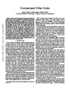
Figure 16 shows the performance comparison of the (7, 4, 3) Hamming code in the AWGN and fading channels. Comparing the performance at 10-4, the MAP-SPC is about 0.3 dB worse than soft decision brute force decoding in the AWGN channel. It is about 1 dB better than hard decision decoding, represented by the hard algebraic bound [52]. In the fading channel, the suboptimality is about 0.6 dB, whereas the gain over hard decoding is about 5 dB. Figure 17 shows the performance of the (15, 11, 3) Hamming code under the same channel conditions. Due to suboptimality, about 0.3 dB and 1.2 dB are lost in the

23 AWGN and fading channels respectively. Gains of about 1.0 dB and 5 dB are achieved over hard decoding. Figure 18 compares the performance of (31, 26, 3) Hamming codes and uncoded BPSK. As in previous cases, the MAP-SPC decoding gains about 0.8 dB and 5 dB over the hard decoding in the AWGN and fading channels respectively. At 10-4, the MAP-SPC decoded Hamming code gains about 2 dB and 17 dB over the uncoded BPSK scheme in the respective channels. The performance of the (63, 57, 3), (127, 120, 3) and (255, 247, 3) Hamming codes are shown in Figure 19, Figure 20 and Figure 21 respectively. In the AWGN channel, there is a slight reduction in the gain over hard decoding from 0.7 dB to 0.6 dB to 0.5 dB, as the code length increases. However, in the fading channel, the gain stays rather consistently at about 5 dB. Figure 22 compares the performance of MAP-SPC with the dual code technique in [30] using a parallel concatenated (7, 4, 3) Hamming code in the AWGN channel. In [30], this code was decoded using the dual code of the (7, 4, 3) Hamming code, which is the (7, 3, 4) maximum length code. After 6 iterations, the MAP-SPC technique is about 0.25 inferior to the dual code technique. The advantage of the MAP-SPC technique is the lower decoding complexity, which is detailed next.

24

(7, 4, 3) Hamming code

0

10

soft brute force decoding hard algebraic bound MAP-SPC (4 it) MAP-SPC (3 it)

-1

10

-2

bit error rate

10

-3

10

-4

10

-5

10

-6

10

-7

10

0

5

10

15 Eb/No

20

25

30

Figure 16 : Performance comparison of the (7, 4, 3) Hamming code in the AWGN (left curves) and fading (right curves) channels.

25


0

10

soft brute force decoding hard algebraic bound MAP-SPC (5 it) MAP-SPC (3 it)

-1

10

-2

bit error rate

10

-3

10

-4

10

-5

10

-6

10

-7

10

0

5

10

15 Eb/No

20

25

30


26


0

10

Uncoded BPSK hard algebraic bound MAP-SPC (7 it) MAP-SPC (5 it)

-1

10

-2

bit error rate

10

-3

10

-4

10

-5

10

-6

10

-7

10

0

5

10

15

20

25

30

35

Eb/No


27


0

10


-1

10

-2

bit error rate

10

-3

10

-4

10

-5

10

-6

10

-7

10

0

5

10

15

20

25

30

35

Eb/No

Figure 19 : Performance of the (63, 57, 3) Hamming code in the AWGN (left curves) and fading (right curves) channels.

28


0

10


-1

10

-2

bit error rate

10

-3

10

-4

10

-5

10

-6

10

-7

10

0

5

10

15

20

25

30

35

Eb/No


29


0

10


-1

10

-2

bit error rate

10

-3

10

-4

10

-5

10

-6

10

-7

10

0

5

10

15

20

25

30

35

Eb/No


30

Product (7, 4, 3) Hamming codes in AWGN

-1

10

MAP-SPC (6 it) MAP dual (6 it)

-2

bit error rate

10

-3

10

-4

10

-5

10

0

1

2

3 Eb/No

4

5

6

Figure 22 : Comparing the performance of the dual code technique [30] and the MAPSPC technique. The code used is the parallel concatenated (7, 4, 3) Hamming code.

31

2.6

Decoding Complexity

The exact decoding complexity will depend on the actual implementation. However, the number of codewords that has to be searched provides a raw complexity estimate [30]. A (n, k, 2) MAP-SPC decoder implemented using its dual code – (n, 1, n) repetition code – requires only 2 codeword searches per iteration. Using this as a complexity measure, the complexity of the MAP-SPC scheme applied to a (N, K) systematic block code is equal to 2*(N-K)*I codeword searches, where I is the number of iterations, K is the data length and N is the code length. One of the most efficient MAP decoding techniques in the literature is the dual code technique as described in [30]. Here, the complexity of the dual code technique is compared to the MAP-SPC. For a (N, K) code, the number of codeword searches required by the dual code method of [30] is equal to 2(N-K) *I. Table 3 provides a comparison of the number of codeword searches required per iteration for both techniques. (Note that the dual SISO method is expected to produce better bit error rate performance compared to the MAP-SPC method. Here, both schemes are compared without taking into account the bit error rate performance.) MAP-SPC

Dual code


6

8


8

16


10

32


12

64


14

128


16

256

Table 3 : Comparison of the number of codeword searches required per iteration for the MAP-SPC and dual code techniques.

From Table 3, it is observed that the complexity of the dual code technique increases exponentially as the code length increases. On the other hand, the complexity of the MAP-SPC technique only increases linearly with increasing block length. Also, each

32 codeword search for the MAP-SPC method is conducted over repetition codes. For example, the MAP-SPC codeword search for the (63, 57, 3) Hamming code is conducted over the (32, 1, 32) repetition code. For the dual SISO technique, the codeword search is conducted over a much more complex codeword. For example, the dual SISO codeword search for the (63, 57, 3) Hamming code is conducted over the (63, 6) block code. Therefore, in effect, the complexity advantage of the MAPSPC technique is much greater than the estimated figures. In general, hard decision syndrome decoding is less complex than the MAP-SPC scheme. For short code lengths, the complexity of soft decision brute force decoding is lower than the MAP-SPC technique. For example, brute force decoding of the (7, 4, 3) Hamming code requires a search over 24 = 16 codewords. The MAP-SPC scheme requires a search over 6 codewords per iteration. Iterated 4 times, this translates to a total of 24 codeword searches. Nevertheless, similar to the dual code comparisons, both searches are conducted over different types of codewords. Also, the complexity of brute force decoding increases exponentially with block length at a significantly faster rate than the dual code technique.

2.7

Convergence of the Decoding Algorithm

Figure 23 shows the convergence behaviour of the MAP-SPC decoding algorithm for the (255, 247, 3) Hamming code in the fading channel. The convergence is stable. It is observed that as the SNR increases, more iterations are required to produce the best performance. At 20.0 dB, there is negligible gain after 6 iterations. However, at 26.0 dB, there is only negligible gains after 9 iterations. Nevertheless, the gain after 5 iterations at all SNR shown is small, perhaps too small to be worth its computation in a practical system. In general, the MAP-SPC decoding algorithm is found to converge quickly in both AWGN and fading channels. This fast convergence is a desirable feature as it results in lower overall decoding complexity and decoding delay.

33 Convergence of (255, 247, 3) Hamming code in fading

-3

10

26.0 dB 25.0 dB 24.0 dB 23.0 dB 22.0 dB 21.0 dB 20.0 dB

-4

bit error rate

10

-5

10

-6

10

1

2

3

4

5 6 number of iterations

7

8

9

10

Figure 23 : Convergence behaviour of MAP-SPC decoding of the (255, 247, 3) Hamming code in the Rayleigh fading channel.

2.8

Summary

In this chapter, an iterative decoding technique based on MAP decoding of single parity check codes is applied to SISO decoding of systematic binary algebraic block codes. The MAP-SPC scheme preforms very well compared to hard decision syndrome decoding and soft decision brute force decoding. The decoding complexity of this scheme grows linearly instead of exponentially with increasing block length. For codes such as Hamming codes, only 1 MAP-SPC decoder is needed to perform the whole decoding process. The component MAP decoders are extremely simple to implement. It can be further simplified by using the approximated Log-Likelihood Algebra (LLA) [30] for implementation on fixed point DSPs (refer to Appendix I for details).

34 In theory, this technique can be applied to any systematic block code. In general, the performance of this decoding strategy is expected to lie between those of ML soft decision decoding and hard syndrome decoding. The additional complexity of the MAP-SPC technique over hard algebraic decoding may or may not be worth the effort in the AWGN channel. On the other hand, a 5 dB gain at 10-4 in the fading channel is achieved by adopting the MAP-SPC technique. This is a significant gain, and is well worth the extra effort. It is well known that the first few dB of gain is simple to achieve. After that, it becomes more difficult to improve performance. Depending on the application, the last minor gains may or may not be of practical interests. With this technique, there is an option to avoid the exponential complexity of a ML soft decoding algorithm at the cost of losing the last minor amount of gain. It is obvious that this technique is suboptimal; concatenated iterative decoding is inherently suboptimal. Despite this suboptimality, this decoding strategy is a strong candidate for SISO decoding of long block codes, a feat not computationally practical for either brute force or trellis-based methods. This has a potential application in the decoding of concatenated block codes. In addition, the work presented here can potentially be used to study the suboptimal performance and convergence behaviour of iteratively decoded codes. Though there is no explicit interleaver within the parallel concatenated encoder structure of Figure 14, the performance of iterative decoded Hamming codes provide an excellent starting point for studying iterative decoder structures, and the iterative decoding performance of short length block codes.

35

CHAPTER 3 : DESIGN, ANALYSIS AND PERFORMANCE OF CONCATENATED SINGLE PARITY CHECK (SPC) CODES

3.1

Introduction

Single parity check (SPC) codes are some of the simplest and weakest algebraic codes in existence. A simple code is inherently simple to decode. Despite its simplicity, it has been shown to produce high performance at low complexity. This chapter presents two concatenated SPC coding schemes to attack the error floor, block length and code rate problems encountered in previous efforts as outlined in Chapter 1. The Two schemes are the multiple parallel and the multiple serially concatenated SPC codes. The dimension of the codes is increased to improve the error performance. The error floor is also pushed further down as the dimensionality is increased. A method of incrementing the number of dimensions without changing the code rate and block length requirements is presented. Analytical bounds for these codes fixed at a rate of ¾ and a data block lengths of 900 bits are derived to estimate the asymptotic performance in the AWGN and independent Rayleigh fading channels. An improved decoder structure for serially concatenated codes is also presented.

36 3.2

Multiple Parallel Concatenated SPC Codes

3.2.1

Encoder Structure

An M parallel concatenated SPC code consists of M SPC encoders, separated by M-1 interleavers. Figure 24 shows the general encoder structure for multiple parallel concatenated single parity check codes (M-PC-SPC). The constituent interleavers can be of any type. In this work, random interleavers are used. The number of parallel concatenations is increased to improve performance. With an input block length of K bits and output block length of N bits, the overall code rate of k/n is retained by selecting the (k*M)/ (k*M+1) SPC as component codes. systematic bits K input bits

(k*M+1, k*M, 2)

Data Block

SPC Encoder 1

parity bits 1

p1

SPC Encoder 2

parity bits 2

p M-1

SPC Encoder M

parity bits M

N output bits

Figure 24 : General encoder structure for Multiple Parallel Concatenated Single Parity Check Codes (M-PC-SPC).

The following example shows how a rate ¾ 3 parallel concatenated SPC (3-PC-SPC) code with a data block length of 900 bits is constructed. The numerator of the overall code rate is multiplied by the number of parallel concatenations, M. In this example, the targeted code rate is ¾. Both the numerator of the targeted code rate and M are

37 equal to 3, so the component SPC is a (3*3)/(3*3+1) SPC code. As a result, the 3-PCSPC code is composed of 3 (10, 9, 2) SPC component codes. This technique can be extended to any code rate and almost any data block size. The only requirement is that the data block size has to be an integer multiple of the component SPC code’s input word length. In the example, any data size that is an integer multiple of 9 can be used.

3.2.2


Figure 25 shows the decoder structure of a 3-PC-SPC code. The component soft-insoft-out (SISO) decoder is shown in Figure 26. Each component decoder accepts soft information (LLR) from the demodulation process. These soft informations are combined with a priori information to generate extrinsic information for each data bit. The generated extrinsic information is then used by other component decoders as a priori information. There is no self-feedback of extrinsic information, meaning that extrinsic information generated by decoder 1 is used only by decoders 2 and 3. Although not explicitly shown in Figure 25, all soft informations are properly interleaved and deinterleaved before being used.

channel LLR

(10, 9, 2) SPC Decoder 1

extrinsic info decoder 1





Figure 25 : Decoder structure for the 3-PC-SPC code.

Hard Decision

38 Channel LLR a priori LLR 1

SISO Component Map Decoder

extrinsic info from decoder

a priori LLR 2

Figure 26 : SISO component MAP unit for each decoder.

The SISO component decoding units perform symbol-by-symbol MAP decoding of SPC codes. The MAP algorithm for SPC codes is shown in Appendix I.

3.2.3

Analytical Bounds

This section provides analytical estimates for the codes’ performance at high SNR. It is not our intention to tackle this difficult bounding problem with rigour here. The analytical bounds employ the Input Redundancy Weight Enumerating Function (IRWEF) based on the work of [32]. The bounds are not very tight, particularly at very low SNR, because the decoding technique is suboptimal whereas the bounds assume ML decoding. Also, due to the computational complexity, only part of the codes’ weight distributions are taken into account. Nevertheless, the work here provides good estimates of where the error floors are, and provides sufficient guidelines for the purpose of practical systems design. Performance bounds for the codes at an input length of 900 bits, output length of 1200 bits, and a code rate of ¾ are shown here. In [53], BER bounds for parallel concatenated SPC codes and zigzag codes were presented. They have used essentially the same approach as the method presented in this section to increase the dimensionality without changing the code rate or block length. The work in this section is a direct extension of [55].

39 3.2.3.1

The Union Bound

In [32], the Input Redundancy Weight Enumerating Function (IRWEF) for a (n, k) linear block code is defined as

AC (W , Z ) = ∑ Aw, jW w Z j w, j

where Aw,j denotes the (integer) number of codewords generated by an input information word of Hamming weight w, whose parity check bits have Hamming weight j, so that the overall Hamming weight is w + j. W and Z are symbolic variables. Under the uniform error property of a linear block code, the word and bit error probability performance of the code can be evaluated under the assumption that the all zero codeword, x0, was transmitted. The pairwise error event e0h(w) is then defined as the event in which the likelihood of a codeword with weight h and generated by an information word of weight w is greater than that of the all zero codeword x0. Using the union bound, the bit error probability under ML soft decoding for BPSK transmission can then be upper bounded as [32]

Pb (e) ≤ ∑ Dh P [e0 h ( w)] h

where Dh is derived from the IRWEF as

Dh =

w A w, j k j + w=h

∑

Clearly, 2 terms have to be computed for the upper bound, namely, the pairwise error event probability and the term Dh.

40 3.2.3.2

Pairwise Error Event Probability

The pairwise error event probability is dependent on the channel. For the AWGN channel, it is equal to [25]

⎛ hRc Eb 1 P [eoh (w)] = erfc ⎜⎜ 2 N0 ⎝

⎞ ⎟ ⎟ ⎠

where Rc = k/n is the code rate. For the independent fading channel, it is approximated as [56]

⎛ ⎡ Eb ⎜ R c N0 1⎜ ⎢ P [eoh ( w)] ≤ ⎜1 − ⎢ E 2⎜ ⎢ 1 + Rc b ⎜ ⎢⎣ N0 ⎝

3.2.3.3

⎤ ⎥ ⎥ ⎥ ⎥⎦

1

2

h −1 ⎞⎛ ⎞ ⎟⎜ ⎟ ⎟⎜ 1 ⎟ ⎟⎜ ⎟ ⎟⎜ 1 + Rc Eb ⎟ ⎟⎝ N0 ⎠ ⎠

The Dh Term

The Dh term can be extracted from the IRWEF of the code. Therefore, the final piece of computation required is the derivation of the IRWEF for M-PC-SPC codes. This derivation is extended to higher dimensionalities (> 3 dimensions) based on the work of [32]. The extension is a simple and straightforward task. The IRWEF computation is included in Appendix II.

3.2.4

Bounds Compared to Simulations Results

The bounds for the M-SPC-SPC codes in the AWGN and independent fading channels using BPSK are presented here using only partial IRWEFs. As mentioned earlier, evaluating the complete IRWEF of the M-PC-SPC codes at an input data block length of 900 bits for 2 to 6 dimensions is an almost computationally impossible

41 task. For practical reasons, only a limited number of terms of the IRWEF is computed. Here, the partial IRWEF of the M-PC-SPC codes are computed using the first 22 terms of the IRWEF of the component codes. Figure 27 compares the bounds for 2, 3, 4, 5 and 6-PC-SPC codes with the simulation results in the AWGN channel. Figure 28 shows the bounds for the same codes in the independent fading channel. The bounds obtained for all the codes provide good estimates in both channels at high SNR. It is interesting to note that both the simulations and bounds indicate that, as the dimensionality of the codes increases from 4 to 5, the error floors are lowered by more than 1 order of magnitude in both channels (≈10-4 to < 10-5 in AWGN at about 3.3 dB, and >10-5 to ≈10-6 in fading at about 9 dB). As the dimensionality increases from 5 to 6, the error floor is lowered by almost 2 orders of magnitude in both channels ( 3 dimensions) based on [25] [27]. The extension is a simple and straightforward task. The IOWEF computation is shown in Appendix III.

3.4.4

Bounds Compared to Simulations Results

The bounds for the 2, 3 and 4-SC-SPC codes in the AWGN and independent fading channels using BPSK are presented here using the partial CWEFs. For practical reasons, the partial CWEF of the M-SC-SPC codes are computed using the first 25 terms of the CWEF of the component codes. Figure 35 shows the bounds for 2, 3 and 4-SC-SPC codes compared to simulation results in the AWGN channel. Figure 36 shows the bounds for the same codes in the independent fading channel. At high SNR, the bounds obtained for the 2, 3 and 4-SCSPC codes are quite good in both channels. We note that, as the dimensionality of the code increases from 3 to 4, the simulations and bounds indicate that the error floors are lowered by approximately 2 orders of magnitude in the AWGN channel (≈10-4 to ≈10-6 at about 4 dB). For the fading channel, the floor is lowered by more than 1 order of magnitude (> 10-5 to < 10-7 in fading at about 11 dB). Analytical bounds for the 5 and 6-SC SPC codes in the AWGN and fading channels are compared in Figure 37 and Figure 38 respectively. The bounds are very loose at low SNR because insufficient terms were evaluated, mainly due to the computational complexity involved. However, they provide some approximation for the asymptotic performance. Simulation results show that the error floor is not present at error rates above 10-6. The bounds suggest that the error floors are pushed to very low error rates (< 10-9).

51

Comparing 2,3 and 4-SC schemes to bounds - AWGN

0

10

2-SC (3 it) 3-SC (5 it) 4-SC (8 it) 2-SC bound 3-SC bound 4-SC bound

-2

10

-4

bit error rate

10

-6

10

-8

10

-10

10

-12

10

2

3

4

5

6 Eb/No

7

8

9

10

Figure 35 : Bounds for 2, 3 and 4-SC-SPC codes with the simulation results in the AWGN channel.

52

Comparing 2,3 and 4-SC schemes to bounds - fading

0

10

2-SC (3 it) 3-SC (4 it) 4-SC (4 it) 2-SC bound 3-SC bound 4-SC bound

-2

10

bit error rate

-4

10

-6

10

-8

10

-10

10

5

10

15

20

Eb/No

Figure 36 : Bounds for 2, 3 and 4-SC-SPC codes with the simulation results in the fading channel.

53

Comparing 5 and 6-SC schemes to bounds - AWGN

0

10

5-SC bound 6-SC bound 5-SC (10 it) 6-SC (10 it)

-2

10

-4

bit error rate

10

-6

10

-8

10

-10

10

-12

10

-14

10

0

1

2

3

4 Eb/No

5

6

7

8

Figure 37 : Bounds (dashed lines) for 5 and 6-SC-SPC codes with the simulation results (solid lines) in the AWGN channel.

54 Comparing 5 and 6-SC schemes to bounds - fading

0

10

5-SC bound 6-SC bound 5-SC (10 it) 6-SC (10 it)

-2

10

-4

bit error rate

10

-6

10

-8

10

-10

10

-12

10

-14

10

0

2

4

6

8

10 Eb/No

12

14

16

18

20

Figure 38 : Bounds (dashed lines) for 5 and 6-SC-SPC codes with the simulation results (solid lines) in the fading channel.

3.5

Summary

In this chapter, it has been shown that, by increasing the dimensionality, the error floors of multiple parallel and multiple serially concatenated SPC codes are lowered. At the same time, the bit error performance improves. All these gains are achieved without changing the rate and block length of the code because the component SPC codes are properly chosen. The input data block length is flexible. For multiple parallel concatenated SPC codes, the size needs only be an integer multiple of the input word length of the constituent SPC encoders. For multiple serially concatenated SPC codes, the data block must be an integer multiple of the outer encoder’s input word length. This flexibility opens up these coding schemes to a wide range of practical applications.

55 Analytical bounds are presented to estimate the performance of concatenated SPC codes at high SNRs. Due to computational complexity, only the partial weights of the concatenated codes are considered. Simulation results for low to medium SNRs are presented to complement the asymptotic estimates of the bounds. Together, they provide sufficent guidelines for practical systems design. More investigations on concatenated SPC codes will be presented in chapter 5 where the performance between the parallel and serial schemes are compared, the decoding complexities are estimated and the convergence of the decoding algorithms are discussed. An improved iterative decoder structure for multiple serially concatenated codes is also presented. The decoder maximizes the sharing of soft information among all decoders to produce superior performance compared to the previously used decoder. Though only results for single parity check codes are presented here, the proposed iterative decoder structure is applicable to other component codes, and also product codes. It is very likely that if the improved iterative decoder is employed, there may still be some potential performance gains at low SNR for the works published in [27] and [43].

56

57

CHAPTER 4 : CODED MODULATION

4.1

Introduction

Coded modulation has come a long way since the days of Ungerboeck. Traditionally, coded modulation treats coding and modulation as a single process by employing techniques such as set partitioning of the signal constellation [57]. Set partitioning has been successfully extended using multilevel codes with multistage decoding (MLC/MSD) [58] [59]. Till this day, this coded modulation structure still reigns as the best in the AWGN channel [60] [54]. However, its performance in the Rayleigh fading channel is not as good. Zehavi is arguably the first to recognise the advantages of separating coding and modulation for application to the Rayleigh fading channel [61] [62]. Coding and modulation were separated by performing bit interleaving before mapping the coded bits onto the signal constellation. His work was generalised to Bit Interleaved Coded Modulation (BICM) by Caire et. al. in [63]. Along the way, a few publications have also emerged in the literature with similar ideas [64] [65], [66]. Consistently, the superiority of separating coding and modulation in the Rayleigh fading channel is reported. In this chapter, an overview of key developments in coded modulation is presented. Strong emphasis is placed on the structure of the coded modulation schemes rather than the error correction scheme employed.

58 4.2

Coding and Modulation Combined

4.2.1

Trellis Coded Modulation and Ungerboeck’s Codes

Convolutional codes [67] and the Viterbi algorithm [68] played key roles lead to the advancement and widespread use of combined coding and modulation. At one stage convolutional codes were considered as the most powerful practical codes. Convolutional codes are more flexible in block length and code rates compared to block codes such as Hamming codes (pre-fixed block length). The Viterbi algorithm provided a way of implementing tractable maximum likelihood soft decision decoding of convolutional codes. In [57], Ungerboeck was first to combine convolutional codes with multilevel signal constellations, forming Trellis Coded Modulation (TCM) [69], [70]. The significance of Ungerboeck’s contribution lies in the use of larger signal constellations to cater for the redundant bits from the error correction codes such that bandwidth efficiency is not sacrificed. Designed for the AWGN channel, TCM employs set partitioning to progressively increase the minimum Euclidean distance between successive subsets. Set partitioning for 16-QAM is shown in Figure 39. The subsets resulting from successive partitioning have increasing intra-subset distance. Because the final subset has a very large intra-subset distance, uncoded bits can be used to select the signal points within this subset. This technique is referred to as Ungerboeck codes [71]. Figure 40 shows the structure of a 16-QAM Ungerboeck code with a bandwidth efficiency of 3 bit/s/Hz. In principle, a rate ¾ convolutional code can also be used to achieve better gain since there are no parallel transitions, though this comes at the expense of increased decoding complexity. TCM using signal constellations of higher dimensions are found in [69] and [70]. Schemes using signal constellations derived from lattice theory are presented in [72], [73], [74], [75] and [76].

59 d0 d3 > d2 > d1 > d0 0

S0/S1

1

d1 0

S1/S2

0

1

1

d2

S2/S3

0

1

0

1

0

1

0

1

d3

Figure 39 : Set partitioning for a 16-QAM signal constellation.

data bits

rate 2/3 Convolutional Code

S0/S1 S1/S2 S2/S3 S3/S4 select signal point

Figure 40 : The structure of a 16-QAM Ungerboeck code with a bandwidth efficiency of 3 bits/s/Hz.

4.2.2

Trellis Coded Modulation for the Rayleigh/Rician Fading Channels

Trellis coded modulation schemes using MPSK modulation were extended to Rayleigh/Rician fading channels by Simons and Divsalar. In [77] the performance criteria were identified. They showed that substantial performance improvement can be achieved using simple TCM schemes combined with interleaving/deinterleaving. Interleaving plays the role of a zero redundancy code that “randomizes” the distribution of the errors, breaking up bursts and destroying the memory of the channel. In [78], optimum code design techniques using set partitioning were

60 presented. Multiple symbols were associated to a trellis branch to form multiple trellis coded modulation (MTCM). It was shown that MTCM is capable of achieving larger diversities than conventional trellis coded modulation. Other TCM efforts for fading channels can be found in [79] and [80].

4.2.3

Multilevel Codes with Multistage Decoding (MLC/MSD)

Multilevel codes were originally invented by Imai and Hirakawa [81] in 1977. Unfortunately, in the early days, this powerful coding structure failed to find much use in practical applications, partly due to the fact that the multiple error correction codes require multiple decoders at the receiver, which was seen as a implementation disadvantage. Also, in [81], only algebraic decoding was considered.

4.2.3.1 Based on Euclidean Distance In 1989, Pottie and Taylor [58] applied multilevel codes to set partitions, resulting in a multilevel partition code, shown in Figure 41. The multistage decoder for this code is shown in Figure 42. At about the same time, this idea was also proposed by [59]. As with TCM, the multilevel partition code maximises the minimum Euclidean distance of successive partitions. The result is a very powerful reduced complexity coding structure. A multilevel concatenated partition code was also proposed to produce better performance [82]. This structure is shown in Figure 43. One work employing this structure is found in [83]. In [84] and [85], multilevel codes for the Rayleigh fading channel were presented. Multilevel codes over geometrically uniform partitions in the Rayleigh fading channel was investigated in [86].

61

data bits

Encoder 1

S0/S1

Encoder 2

S1/S2

Encoder 3

S2/S3

Encoder 4

S3/S4 select signal point

Figure 41 : Multilevel code with set partitioning (multilevel partition code).

Decoder 1 Decoder 2

Channel Output

Decision Making

Decoder 3 Decoder 4

Figure 42 : Multistage decoder (MSD) for a multilevel partition code.

GF(2q)

Encoder 1

S0/S1

Encoder 2

S1/S2

Encoder B

Encoder 3

S2/S3

Encoder C

Encoder 4

S3/S4

Encoder A data bits

GF(2)

select signal point Figure 43 : Multilevel concatenated partition code.

62 4.2.3.2 Based on Equivalent Channel Capacities Huber et. al. [87], [88], [89], [90] and Kofman et. al. [91], [92], independently proved that the capacity of a modulation scheme can be achieved by multilevel codes with multistage decoding if and only if the individual rates of the component codes are properly chosen. This was proven using the chain rule for mutual information [93] [94]. The chain rule provides a model with virtually independent parallel channels for each address bit at the different partitioning levels, called equivalent channels. The equivalent channel represents the channel as “seen” by each partition/encoder. The information theoretic parameters of these channels lead to theoretical statements and practical rules for designing and constructing coded modulation schemes [90]. Figure 44 shows the structure of this coding scheme. In the figure, rk denotes the code rate of encoder k, and Ck denotes the channel capacity of the respective equivalent channels.

Encoder 1 data bits

Encoder 2 Encoder 3 Encoder 4

r1 = C1 r2 = C2 r3 = C3

Mapping/ Partitioning

r4 = C4

Figure 44 : Multilevel codes designed with equivalent channel capacities.

4.3

Coding and Modulation Separated

4.3.1

I-Q Trellis Coded Modulation

This form of TCM is the first small step towards the departure from Ungerboeck’s paradigm. I-Q TCM involves splitting a 2 dimensional modulation scheme into 2 independent 1 dimensional modulations, represented by the in-phase and quadrature components. This is shown in Figure 45.

63

Encoder

In-Phase Mapping onto Signal Constellation

data bits Encoder

Quadrature

Figure 45 : Structure of an I-Q TCM scheme.

The idea of I-Q TCM first appeared in “pragmatic” TCM design by Viterbi et. al. [95]. Their scheme used 2 off-the-shelf rate ½ 64-state encoders to encode the inphase and quadrature components of a QAM constellation. This approach results in quadrupling the QAM constellation over what is required over uncoded transmission. For example, to achieve a bandwidth efficiency of 2 bits/s/Hz, 16-QAM is required for the pragmatic scheme compared to 4-PSK for the uncoded scheme. In [96], Heegard et. al. uses off-the-shelf convolutional codes with QAM modulation and demonstrated how coded QAM modulation can be implemented using QPSK-based coded modulation. This was shown to eliminate the need to quadruple the signal constellation size. In [97], the I-Q approach was used for transmitting 2 bits/s/Hz on the Rician fading satellite channel. In [98], the performance of I-Q TCM with 2 parallel 4-state encoders was compared the that of an 8-state 8-PSK trellis code. A large coding gain in the Rayleigh fading channel is achieved by using IQ-TCM. In [64], generalisation of these previous works are presented for spectral efficiencies of 1, 2 and 3 bits/s/Hz. Comparison to conventional TCM using convolutional codes of different constraint lengths show that I-Q TCM schemes offer a significant performance advantage in the Rayleigh fading channel.

4.3.2

Zehavi’s Bit Interleaving Coded Modulation (Multiple Interleavers)

Bit interleaved coded modulation as we know it today was originally proposed by Zehavi in [61]. In the paper, Zehavi constructed a coded modulation scheme employing a rate 2/3 convolutional code with 8-PSK. The novelty of his work lies in the use of 3 bit interleavers instead of 1 symbol interleaver prior to mapping the coded bits to modulation symbols. The symbol interleaver and bit interleaver schemes are shown in Figure 46 and Figure 47 respectively. His work has shown that, compared to

64 symbol interleaving, bit interleaving produces superior performance in the Rayleigh fading channel because the diversity of the coded modulation scheme is increased. His work was extended by Kofman [62], [92] to multilevel codes designed using equivalent channel capacities, shown in Figure 48. Each equivalent channel is encoded by a separate encoder.

data bits

rate 2/3 Convolutional Encoder

Symbol Int

8-PSK Mapping

Figure 46 : Conventional coded modulation with symbol interleaving.

data bits

bit int 1 bit int 2 bit int 3


8-PSK Mapping

Figure 47 : Zehavi's coded modulation design using 3 bit interleavers.

Encoder 1 data bits

Encoder 2 Encoder 3

r1 = C1 r2 = C2 r3 = C3

bit int 1 bit int 2 bit int 3

8-PSK Mapping

Figure 48 : Kofman's extension of Zehavi's work to multilevel codes.

4.3.3

Channel Symbol Expansion Diversity (CSED)

In [99], [100], [65], channel symbol expansion diversity (CSED) was proposed. Traditionally, in order to achieve the same bandwidth efficiency as an uncoded system, a 2-fold signal constellation expansion is used to offset for the redundant bits due to coding. For example, to achieve 2 bits/s/Hz, a typical uncoded system uses 4PSK whereas Ungerboeck’s approach would employ 8-PSK with a rate 2/3 code.

65 Hansson’s proposal employs a 4-fold signal constellation expansion5. In his work, 16QAM was used with a rate 2/4 code to achieve a bandwidth efficiency of 2 bits/s/Hz. Zehavi’s bit interleaving was also used in his scheme to increase the code diversity. Hansson’s results show that, in the Rayleigh fading channel, the 4-fold expansion scheme performs better than the 2-fold expansion scheme due to the increased code diversity of the rate 2/4 code.

4.3.4

Multilevel Codes with Independent Decoding on Levels (MLC/IDL)

The multistage decoder for multilevel codes designed using the equivalent channel capacities method was shown to be the optimum decoder structure [87] [88]. Unfortunately, the optimality only applies to the asymptotic case (i.e. optimum for codes of infinte length). For finite codeword lengths, there is inherent error propagation in the multistage decoder which may lead to a significant performance degradation. In [66], an alternative decoding structure for multilevel codes was proposed to overcome the error propagation problem. Independent decoding on levels (also known as parallel decoding of levels) avoids the error propagation by treating each level separately. The decoder structure is shown in Figure 49.

Decoder 1 Channel Output

Decoder 2 Decoder 3

Decision Making

Decoder 4 Figure 49 : The decoder structure for multilevel codes with independent decoding on levels (MLC/IDL).

Although the MLC/IDL scheme in [66] uses symbol interleaving instead of bit interleaving, an analogous effect to bit interleaving is achieved. This is because each 5

Note that this idea can be traced back to earlier pragmatic I-Q TCM efforts such as the work of

Viterbi [95]. The subtle difference is that Viterbi used 2 encoders whereas Hansson used only 1 encoder.

66 level is comprised of a different encoder and at the decoder, the separate decoders in each level produces the independence effect similar to a bit interleaving scheme. Schramm demonstrated via simulations that MLC/IDL produces the best overall performance when compared to MLC/MSD in both the AWGN and Rayleigh fading channels. A variant of multilevel coding based on Multiple Classes of Levels was considered for an evolved GSM and IS-136 system in [101].

4.3.5

Caire’s Bit Interleaved Coded Modulation (Single Interleaver)

Zehavi’s multiple interleaver bit interleaving scheme was generalised by Caire et. al. in [102], [63]. Instead of using separate bit interleavers for the encoder output, all the bit interleaving is performed by only 1 bit interleaver, resulting in Bit Interleaved Coded Modulation (BICM). A BICM scheme using a rate ¾ convolutional code with 16-QAM is shown in Figure 50. Using a single interleaver, the BICM scheme can be modelled using the equivalent parallel channel model shown in Figure 51 [63]. Extensive analysis performed in [63] shows the superiority of BICM in the Rayleigh fading channel. The work of [90] mentions the similarities between BICM and MLC/IDL.

data bits


Bit Int

16-QAM Gray Mapping

Figure 50 : Caire's single interleaver bit interleaving scheme, generalised from Zehavi's multiple interleaver scheme.

67 Binary Input Channel 1

data bits

Encoder

Parallel to Serial

Binary Input Channel 2 Binary Input Channel 3 Binary Input Channel 4

Figure 51 : Equivalent parallel channel model for a 16-QAM BICM scheme.

4.4

Coded Modulation Employing Turbo Codes

Since the invention of Turbo codes, there have been numerous efforts to incorporate Turbo codes into coded modulation. The first attempt to employ Turbo codes in a pragmatic approach to TCM was the work of [18]. Soon after that, Turbo codes were applied as component codes in multilevel codes [103]. Using the equivalent channel capacity technique applied to multilevel codes with multistage decoding, the performance of 8-PSK, 16-QAM, 32-QAM and 64-QAM in the AWGN was shown to be less than 1 dB away from the AWGN channel capacity using blocklengths of 20,000 bits. The work of [104] and [105] introduced the idea of iterative multistage decoding. Turbo Trellis Coded Modulation (TTCM) schemes were proposed in [106], [107], [108], [109], [110]. Parallel and serial concatenated TCM schemes were reported in [111] and [112] respectively. More recent implementations of turbo codes with bit interleaved coded modulation are found in [113], [114], [115], [60], and [116].

68

4.5

Summary

An overview of key developments in coded modulation has been presented in this chapter. Bit interleaved coded modulation (BICM) is a relatively new scheme. While BICM has been shown to be inferior to multilevel coding in the AWGN channel [90], various works in the literature consistently suggest that separating coding and modulation increases the code diversity effect, and therefore, it is advantageous in the Rayleigh fading channel [61] [60]. Because the channels encountered in practical mobile systems are mostly of the Rayleigh type, it is suggested that BICM may be a practical solution. As the primary of interests of this thesis is the Rayleigh fading channel, the work in subsequent chapters employs BICM with simple concatenated coding schemes.

69

CHAPTER 5 : PERFORMANCE OF CONCATENATED SINGLE PARITY CHECK CODES WITH BIT INTERLEAVED CODED MODULATION

5.1

Introduction

In this chapter, all the codes designed in Chapter 3 are extended to BICM. The error performance of Symbol Interleaved Coded Modulation (SICM) and Bit Interleaved Coded Modulation (BICM) are compared in the independent Rayleigh fading channel. The performance of all the parallel and serially concatenated SPC codes are compared using BICM, and then benchmarked against the best schemes in the literature. Decoding complexity estimates are provided for both schemes. Convergence of the decoding algorithms is also discussed.

5.2

System Model

Figure 52 shows the system model being considered. All the channel coding schemes used in this chapter has the same input data block of 900 bits and output block length

70 of 1200 bits, resulting in an overall code rate of ¾. For BICM, a random bit interleaver precedes the mapping process order to scramble the bit mappings onto the channel symbols. For SICM, this bit interleaving process is omitted. The AWGN and the independent Rayleigh fading channels are considered here. At the receiver, we have assumed that coherent demodulation is performed with the presence of perfect channel state information. After computing the metrics, the minimum metrics are selected and then deinterleaved to reverse the effect of the bit interleaving. The decoder accepts the deinterleaved metrics and starts the decoding process. The MAP algorithm for SPC codes in Appendix I is used.

data encoder

bit interleaver

16-QAM mapping channel

data decoder estimate

metric deinterleaver

demodulation

Figure 52 : System model .

The coded bits are transmitted using gray mapped 16-QAM as in Figure 53. In both the AWGN and Rayleigh fading channels, the demodulation process is performed by treating 16-QAM as 2 independent 4-ASK channels [117] as shown in Figure 54. Two separate sets of the metric are computed. The first set is computed using the real part of the received sample and the 4 amplitude levels of the in-phase channel, whereas the second set is computed using the imaginary part of the received sample and the 4 amplitude levels of the quadrature channel. With 16-QAM, the received sample is compared to all 16 symbols on the signal constellation. With 4-ASK, the received sample is compared to 4 symbols on each 4-ASK channel, which sums up to a total of 8 symbols because there are 2 channels (in-phase and quadrature). This reflects a 50% saving in demodulation complexity6. The squared Euclidean distance metric for 4ASK is 1 dimensional whereas the metric is 2 dimensional for 16-QAM. This results in a further reduction in demodulation complexity. Overall, the total complexity of the

6

By demodulation complexity, we are referring to the complexity of the entire metric computation

process.

71 demodulation process is less than half of the demodulation complexity of standard 16QAM.

Quadrature 0100

1100

1000

0000

0110

1110

1010

0010

0111

1111

1011

0011

0101

1101

1001

0001

In-phase

Figure 53 : Gray mapped 16-QAM signal constellation.

Quadrature 00

01

11

10

00

10

In-phase 11

01

Figure 54 : Splitting the gray mapped 16-QAM constellation into 2 independent gray mapped 4-ASK constellations.

5.3

BICM versus SICM

5.3.1

Equivalent Parallel Channel Model

In [63], the concept of an equivalent parallel channel model for BICM systems was presented. This is shown in Figure 55 for the Gray mapped 16-QAM signal constellation. For 16-QAM, each signal point represents 4 bits. Each bit position sees a slightly different channel. Both BICM and SICM can be represented using the parallel channel model of Figure 55. The only difference is that in SICM, each bit

72 position is fixed to 1 of the 4 parallel channels, whereas in BICM, consecutive bits hop randomly among all parallel channels as determined by the random bit interleaver. The correlation effect caused by the modulation process through the use of a fixed channel (ie SICM) is broken by channel hopping, thereby increasing the code diversity.

0100

1100

1000

0000

0110

1110

1010

0010

0111

1111

1011

0011

Most Significant Bit Position 0

Least Significant Bit Position 0

1

0

Legend Decision Boundary Bit = 0 Bit = 1

0101

1101

1001

0001

Figure 55 : The equivalent parallel channel model for a Gray mapped 16-QAM signal constellation.

5.3.2

Performance Comparison

The channel codes used in the SICM and BICM comparisons are the 3 and 4 dimensional parallel concatenated (3-, 4-PC) single parity check (SPC) codes. The code structures are shown in Figure 56 and Figure 57 respectively. Random interleavers are used in the encoders.

73 systematic bits

900 data bits

(10, 9, 2) SPC Encoder 1

parity bits 1

100 p1 parity bits

p1


parity bits 2

100 p2 parity bits

p2


parity bits 3

100 p3 parity bits

900 data bits Data Block

Figure 56 : Encoder structure 3-PC-SPC.

systematic bits

900 data bits


parity bits 1

75 p1 parity bits

p1


parity bits 2

75 p2 parity bits

p2


parity bits 3

75 p3 parity bits

p3


parity bits 3

75 p3 parity bits

900 data bits Data Block

Figure 57 : Encoder structure for 4-PC-SPC.

Figure 58 compares the performance of SICM and BICM in the Rayleigh fading channel with 16-QAM using the 3-PC SPC code. At low SNR, BICM gains about 0.6 dB over SICM. However, at high SNR, the gap increases significantly to more than 4 dB at 5 x 10-6. A closer look at the code structure of the 3-PC-SPC code structure employed in the simulation reveals that this huge gain is not entirely contributed by the BICM interleaver. It was discovered that bad random interleavers used for the 3PC-SPC code structure was the primary reason. Thus, good interleaver design is essential in designing codes for the fading channel.

74 Comparing BICM and SICM using 3-PC

-2

10

3-PC 16-QAM BICM (6 it) 3-PC 16-QAM SICM (6 it)

-3

bit error rate

10

-4

10

-5

10

-6

10

10

11

12

13

14

15 Eb/No

16

17

18

19

20

Figure 58 : Comparing SICM with BICM in the fading channel using 3-PC-SPC.

To show this effect, better random interleavers are used. Figure 59 shows the performance of SICM and BICM using better random interleavers. It is observed that the flooring effect seen previously for the SICM case is not present. This implies that that BICM’s superiority over SICM is largely dependent on the type of channel coding employed. If the channel coding scheme has properly designed bit interleaving, then the resultant gap between SICM and BICM will be small. This marginal gain is also reported in [66]. Although the gain is marginal, BICM appears to always be better than SICM in the fading channel. These results also imply that BICM is capable of compensating to some extent for a badly designed channel coding scheme (i.e. poor random interleaver).

75

-2

Comparing BICM and SICM using 3-PC with "better" random interleaver

10

3-PC 16-QAM BICM (6 it) 3-PC 16-QAM SICM (6 it) -3

10

bit error rate

-4

10

-5

10

-6

10

-7

10

10

11

12

13

14 Eb/No

15

16

17

18

Figure 59 : Comparing SICM and BICM in the fading channel using 3-PC-SPC with “better” random interleaver.

5.4

Performance of Multiple Parallel Concatenated SPC Codes

In this section, simulation results for M = 2, 3, 4, 5 and 6 dimensional PC-SPC structures are presented. The component codes for each scheme and the minimum Hamming distance of the overall code are summarised in the Table 4. Figure 60 shows the performance of these codes in the AWGN channel. The number of decoding iterations used in each curve represents the near-best performance, where further iterations result in little or no gain. In general, the curves show performance improvements and the lowering of error floors with an increasing number of parallel concatenations. By increasing the number of parallel concatenations, the minimum Hamming distance of the code improves, and therefore, the error floor effect is gradually lowered. The 4-PC scheme is the best scheme at 10-4. At 10-5, 5-PC gives

76 the best performance. At 10-6 and beyond, the 6-PC scheme yields the best performance. M-PC-SPC

Component SPC

Minimum Hamming

Coding Scheme

Code

Distance

2-PC-SPC

(7, 6, 2)

3

3-PC-SPC

(10, 9, 2)

4

4-PC-SPC

(13, 12, 2)

5

5-PC-SPC

(16, 15, 2)

6

6-PC-SPC

(19, 18, 2)

7

Table 4 : M-PC-SPC schemes being investigated.

Comparing all M-PC schemes, 16-QAM, AWGN

-1

10

2-PC (4 it) 3-PC (4 it) 4-PC (5 it) 5-PC (5 it) 6-PC (8 it)

-2

10

-3

bit error rate

10

-4

10

-5

10

-6

10

-7

10

-8

10

5

5.5

6

6.5

7

7.5

8

8.5

Eb/No

Figure 60 : Performance of 2, 3, 4, 5 and 6-PC-SPC using 16QAM in the AWGN channel.

Figure 61 shows the performance of the same codes in the Rayleigh fading channel. There is clear evidence of an increasing diversity effect as the number of concatenations increases. Again, this is due to the increasing minimum Hamming

77 distance. Because the minimum Hamming distance of the M-PC-SPC code is equal to M+1, the slope of the BER curve steepens with increasing M prior to the floor effect. Comparing all M-PC schemes, 16-QAM, fading

-2

10

2-PC (4 it) 3-PC (4 it) 4-PC (5 it) 5-PC (5 it) 6-PC (8 it)

-3

10

-4

bit error rate

10

-5

10

-6

10

-7

10

-8

10

10

10.5

11

11.5

12

12.5 Eb/No

13

13.5

14

14.5

15

Figure 61 : Performance of 2, 3, 4, 5 and 6-PC-SPC using 16-QAM in the independent fading channel.

5.5

Performance of Multiple Serially Concatenated SPC Codes

Simulation results for M = 2, 3, 4, 5 and 6 are presented here. As with the parallel concatenated SPC codes, all M-SC-SPC codes are designed with an input data block length of 900 bits with an output code length of 1200 bits, resulting in an overall code rate of ¾. The component codes for each scheme are shown in Table 5. Figure 62 shows the performance of 2, 3, 4, 5, and 6-SC-SPC using 16-QAM BICM codes over the AWGN channel. Again, graphs are plotted using the near best number of decoding iterations. The figures show improved performance at low bit error rates with increasing dimensionality. Above 10-5, the 4-SC-SPC code is the best scheme.

78 Below that, 5-SC-SPC is the superior scheme. The performance of the same codes in the independent fading channel is shown in Figure 63. A similar trend in performance improvements is observed as the dimensionality increases. The 4-SC-SPC code is the best scheme above 10-6. Below that level, the 5-SC-SPC code is the best. 6-SC is expected to dominate only at very low bit error rates. M-SC-SPC

Component SPC

Coding Scheme

Code

2-PC-SPC

(7, 6, 2)

3-PC-SPC

(10, 9, 2)

4-PC-SPC

(13, 12, 2)

5-PC-SPC

(16, 15, 2)

6-PC-SPC

(19, 18, 2)

Table 5 : M-SC-SPC schemes considered.

Comparing all M-SC-SPC schemes, 16-QAM, AWGN

-1

10

2-SC (3 it) 3-SC (5 it) 4-SC (8 it) 5-SC (9 it) 6-SC (10 it)

-2

10

-3

bit error rate

10

-4

10

-5

10

-6

10

-7

10

5

5.5

6

6.5

7

7.5

Eb/No

Figure 62 : 2, 3, 4, 5 and 6-SC-SPC codes using 16-QAM in the AWGN channel.

79

-1

Comparing all M-SC-SPC schemes, 16-QAM, fading

10

2-SC (3 it) 3-SC (5 it) 4-SC (5 it) 5-SC (10 it) 6-SC (10 it)

-2

10

-3

bit error rate

10

-4

10

-5

10

-6

10

-7

10

-8

10

10

10.5

11

11.5 12 Eb/No

12.5

13

13.5

Figure 63 : 2, 3, 4, 5 and 6-SC SPC codes using 16-QAM in the independent fading channel

5.6

Performance Comparison and Benchmark

Table 6 compares the performance of parallel and serially concatenated SPC codes against the best schemes available in the literature at 10-4. The 4-PC and 4-SC code are used for comparison since they achieve the best BER performance at 10-4 among all the parallel and serially concatenated SPC codes considered. All schemes have identical code parameters; code rate is ¾, data block length is 900 bits and the modulation scheme is 16-QAM. From Table 6, the 4-PC code is the best among all the codes in the fading channel. In the AWGN channel, it is second only to the AWGN multilevel 16-state Turbo code. The inferior performance of BICM compared to MLC/MSD is as predicted by [90]. It outperforms the 16-state BICM Turbo code by 0.1 dB in both channels. Moreover, this is achieved with only 5 iterations

80 compared to 6 iterations for the Turbo code. There is a gain of about 0.3 dB and 0.5 dB over the 4-SC code in the AWGN and fading channels respectively. Both the 4-PC and 4-SC codes scheme perform better than the best 64-state multilevel convolutional codes in both channels. Fading

AWGN

Channel

Channel

12.2 dB

8.2 dB

> 14.0 dB

7.0 dB

12.1 dB

6.0 dB

10.9 dB

6.5 dB

4-SC-SPC code – 5 iterations

11.3 dB

6.7 dB

4-PC-SPC code – 5 iterations

10.8 dB

6.4 dB

Best 64-state punctured convolutional codes with MLC/MSD designed for fading channel [101] Best 64-state punctured convolutional codes with MLC/MSD designed for AWGN channel [101] 16-state Turbo codes with MLC/MSD designed for AWGN channel – 6 iterations [60] 16-state Turbo codes with BICM – 6 iterations [60]

Table 6 : Performance comparison of the best schemes in literature at BER = 10-4.

Figure 64 compares the performance of 3-PC, 4-PC with 3-SC and 4-SC at a wider range of bit error rates in the fading channel. The performance curves show that 3-PC is slightly superior to 3-SC above 10-3. However, as the bit error rate moves below 10-4, 3-SC becomes superior. Above 10-5, the 4-PC is the better scheme. However, as the error rates decrease further, the 4-PC scheme hits an error floor before the 4-SC scheme does. Below 10-5, the superiority of 4-SC is not matched by the 4-PC scheme.

81 Comparing 3-SC, 4-SC, 3-PC and 4-PC in fading

-2

10

3-PC (4 it) 4-PC (5 it) 3-SC (5 it) 4-SC (5 it) -3

bit error rate

10

-4

10

-5

10

-6

10

10

10.5

11

11.5

12 Eb/No

12.5

13

13.5

14

Figure 64 : Comparison of 3-SC, 4-SC, 3-PC and 4-PC in the Rayleigh fading channel.

5.7

Decoding Complexity

The decoding complexity of any decoding algorithm varies with different implementation methods and trade-offs. In this section, a rough estimate of the decoding complexity for the 4-PC-SPC code is provided. The complexity is compared to those of Turbo codes and convolutional codes. An approximate per-data-bit Viterbi decoding complexity of a rate ½ convolutional code is given by [15] Cconv = 3S

82 where S represents the number of states in the trellis. In [15], the Log-MAP decoding complexity of the rate 1/3 Turbo code was estimated7. Here, the per-data-bit LogMAP decoding complexity of the Turbo code is approximated using only the dominant factor CTurbo = 18SI where S represents the number of states of the component convolutional codes and I represents the number of decoding iterations. The complexity figures reflect the approximate number of comparison, multiplication and addition operations. This can be used to compare the decoding delays when implemented on a DSP. We note here that operations required for interleaving/deinterleaving of LLRs and other housekeeping operations are not included in this comparison. The decoding complexity of the 4-SC-SPC code is estimated to be about 33 operations per data bit per iteration. After 5 iterations, the total decoding complexity is 165 operations. A 64-state convolutional code requires a total of 192 operations, whereas the 16-state Turbo code (iterated 5 times) requires 1440 operations. The 4SC-SPC code is slightly less complex than the 64-state convolutional code. Compared to the 16-state Turbo codes, it is about 9 times less complex. The decoding complexity of concatenated SPC codes is roughtly proportional to the length of their component SPC codes. In comparison to the 4-SC code, the 4-PC code is about 10% less complex because of shorter component SPC codes – (13, 12, 2), (14, 13, 2), (15, 14, 2) and (16, 15, 2) SPC codes for the 4-SC code as compared to four (13, 12, 2) SPC codes for the 4-parallel concatenated SPC code. Using the 4-SC scheme as a baseline for comparisons, the 4-PC scheme requires about 30 operations per data bit per iteration. This is approximately 10 times less complex than the 16state Turbo code.

7

The Turbo code considered in [60] is basically a rate 1/3 scheme, with appropriate puncturing to give

the targeted code rate. A punctured trellis has the same trellis complexity as a non-punctured trellis. Therefore, we can estimate the decoding complexity of a punctured Turbo code using the rate 1/3 Turbo code.

83 5.8

Convergence of the Decoding Algorithm

The performance curves presented in previous figures represent the near-best achievable performances respectively. This means that further decoding iterations will result in only slightly better performances. Figure 65 shows the convergence characteristics of the decoding algorithm for the 4-PC code in the fading channel. The convergence is smooth and does not exhibit any instability. Smooth convergence is observed in all parallel concatenated SPC codes investigated in this work. It is observed that the optimum number of iterations varies with SNR. At 10.0 dB, there are still small gains abtained if the decoding is pushed beyond 5 iterations. However, at 15.0 dB, there is virtually nothing to be gained beyond 3-4 iterations. Fast and stable convergence are both very desirable properties.

Convergence of 4-PC in fading

-1

10

15.0 dB 14.0 dB 13.0 dB 12.0 dB 11.0 dB 10.0 dB

-2

10

-3

bit error rate

10

-4

10

-5

10

-6

10

-7

10

1

2

3

4


7

8

9

10

Figure 65 : Convergence characteristics of the decoding algorithm of 4-PC in the fading channel.

84 M-SC-SPC codes show negligible or no convergence problems in the AWGN channel. However, in the fading channel, some convergence problems begin to surface for 4, 5 and 6-SC-SPC codes. Based on our simulations, the most severe case appears to be the 4-SC-SPC, shown in Figure 66. It is observed that the bit error rate may get worse as the number of iterations is increased. The decoding algorithm starts to exhibit some instability below 10-5 at around 12.0 dB after 9 iterations. We note that if the suboptimum decoder structure for serially concatenated codes is used, simulation results have shown that the convergence problem becomes more severe. The convergence behaviours are not yet understood at this time.

Convergence of 4-SC in fading

-1

10

13.5 dB 13.0 dB 12.5 dB 12.0 dB 11.5 dB 10.5 dB

-2

10

-3

bit error rate

10

-4

10

-5

10

-6

10

-7

10

1

2

3

4


7

8

9

10

Figure 66 : Convergence of the 4-SC-SPC code in the fading channel using the improved decoder structure.

85

5.9

Summary

The performance of SICM and BICM is compared in the independent Rayleigh fading channel. Simulation results here show that the superiority of BICM over SICM is dependent on the type of channel coding employed. Nevertheless, results show that the extra interleaving provided by the BICM produces an error performance that is always better than SICM in the independent Rayleigh fading channel. With proper code (interleaver) design, the gain of BICM is marginal. Also, BICM is capable of partially compensating for badly designed interleavers within the code structure. The performance of concatenated SPC codes compares very favourably to other schemes in the literature. At 10-4, the 4-PC code outperforms the best multilevel convolutional codes and is only inferior to the AWGN multilevel 16-state Turbo codes in the AWGN channel. Based on the work in this chapter, it can be concluded that there is no single concatenated SPC coding scheme that offers the best performance for every bit error rate. The parallel codes are superior at medium to low BER. Beyond that, they start to encounter error floors and the serial codes begin to show superiority. Decoding complexity estimates for concatenated SPC codes are provided. Based on the estimates, concatenated SPC codes are shown to have significant complexity advantages over Turbo codes. The decoding algorithm for concatenated SPC codes exhibits fast convergence. Convergence is smooth for all parallel concatenated codes investigated. However, in the fading channel, 4, 5, and 6-SC SPC codes exhibit some instabilities. One interesting observation is that the decoding algorithm converges properly up to the first 5 iterations. Therefore, a simple solution to the convergence problem is to limit the decoding to 5 iterations. Even if there is no convergence problem, it would be wise to stop decoding at about 4-5 iterations because additional iterations produce only slight improvement in performance.

86

87

CHAPTER 6 : A GENERALISED PERFORMANCE BOUNDING TECHNIQUE FOR BICM SYSTEMS IN THE RICIAN

FADING CHANNEL

6.1

Introduction

In [63], Caire et. al. presented a comprehensive analysis of BICM in the AWGN and the Rician fading channel. Asymptotic bounds for BICM schemes in the independent Rayleigh fading channel was derived using the BICM Expurgated bound. In this chapter, a generalised performance bounding technique for BICM systems in the Rician fading channel is presented. By using the difference between the BICM Expurgated bounds, it is possible to accurately estimate the error performance of coded BICM systems with larger signal constellations using only the error performance of a BPSK system employing the same channel coding scheme in the same channel. Also, this method is shown to be valid for a wide range of SNR, and to be independent of the type of channel coding scheme and code rate employed. Our work implies that, in the Rician fading channel, analytical bounds for any coding scheme derived for the BPSK system can be easily applied to BICM systems with larger signal constellations in the same channel. In fact, the difference in error

88 performance is merely a translation factor along the SNR (per bit) axis of the bit error rate vs SNR (per bit) plot. Simulation results are presented to verify the analysis. As an introduction to the derivation, Sections 6.1 and 6.2 are directly referenced from [63]. The authors of [63] have performed a comprehensive bounding effort for BICM systems. Sufficient details are provided here to follow the derivations. The interested reader is directed to [63] for a more rigorous treatment. Our derivation begins in section 6.3.

6.2

BICM Expurgated Bound

In [63], the BICM union bound on the bit error probability is defined as

Pub ≤ m − d ∑ 2 − d ∑ 2 − d ( m−1) S

U

∑ ∑ P( x → z )

….(1)

x∈Χ cS z∈Χ cSˆ

where

x denotes the transmitted sequence z denotes the erroneous sequence

P( x → z) is the pairwise error probability between the two signal sequences x and z m denotes the number of information bits represented by a signal point on the constellation d denotes the Hamming distance of the error event X denotes the choice of signal constellation and

X cS = X ci11 × ⋅ ⋅ ⋅ ⋅ × X cikk × ⋅ ⋅ ⋅ ⋅ × X cidd

X cˆS = X cî11 × ⋅ ⋅ ⋅ ⋅ × X cîkk × ⋅ ⋅ ⋅ ⋅ × X cîdd denote the sequence (Cartesian product) of signal subsets selected by the bits c k of

c (correct subsets) and cˆk of cˆ (complementary subsets) given the label positions Sk = ik and the labelling map selected by Uk. S and U range over all the possible m d and 2d sequences of the bit positions of the signal points and constellation mapping respectively.

89 This bound is very loose. To get a tighter bound, it is expurgated to produce the BICM Expurgated bound

Pex ≤ m − d ∑ 2 − d ∑ 2 − d ( m −1) S

U

∑ P( x → zˆ)

….(2)

S

x∈Χ c

where zˆ is the unique nearest neighbour of x in

X zˆS .

The BICM Expurgated bound is similar in form to the BICM union bound, but it includes only one (the nearest) error event ( x → zˆ) for each possible transmitted sequence x , rather than all the possible 2d ( m−1) error events ( x → z) , for all z ∈ Χ cSˆ . It has been shown [63] to provide a tighter approximation to the probability of error. To obtain a computationally efficient form of the BICM expurgated bound, the Laplacetransform approach is used. Using this approach, the expurgated bound is approximated by the Chernoff bound [63] as

Pex ≤ min [ψ ex (α )]d 0

on concatenated single parity check codes and bit

on concatenated single parity check codes and bit

Suggest Documents

Design of Multiple Serially Concatenated Multiple Parity-Check Codes

Soft-Bit Decoding of Regular Low-Density Parity-Check Codes

Turbo Equalization With Single-Parity Check Codes and Unequal ...

Concatenated Low-Density Parity-Check and BCH Coding System for ...

Complexity-Optimized Low-Density Parity-Check Codes

Analysis of Low-Density Parity-Check codes based on

A TUTORIAL ON LOW DENSITY PARITY CHECK CODES

A TUTORIAL ON LOW DENSITY PARITY CHECK CODES

On ensembles of low-density parity-check codes

Concatenated Polar Codes - arXiv

Low-density parity-check codes: Design and decoding - CiteSeerX

Low density parity check codes over groups and rings - CiteSeerX

Bit-error rate analysis of low-density parity-check codes ... - IEEE Xplore

bit, (32,8) CMOS Analog Low-Density Parity-Check Decoder

Introducing Low-Density Parity-Check Codes - Signal Processing ...

Serial Genetic Algorithm Decoder for Low Density Parity Check Codes

Quasi-Cyclic Low-Density Parity-Check Codes for ... - Semantic Scholar

Parity-Check Density versus Performance of Binary Linear Block Codes

Low-density parity-check codes for digital subscriber lines - CiteSeerX

Newly Designed Quasi-Cyclic Low Density Parity Check Codes

Using low density parity check codes in the McEliece ... - CiteSeerX

Decoding low-density parity check codes with normalized APP-based ...

Multiple rate low-density parity-check codes with constant ... - CiteSeerX

Efficient encoding of low-density parity-check codes - CiteSeerX