path from any point A to any other point B from a network T holds, that it is congruent to the path from the point A B to the point 0 = (0;0;:::;0):. 8A; B 2 T : P(A; B) !
Optimal Broadcasting in Toroidal Networks Izidor Jerebic, Roman Trobec Department for Computer Networks and Digital Communications Jo�zef Stefan Institute, Jamova 39 61 111 Ljubljana, Slovenia
Abstract
In this paper we study routing algorithms for broadcasting (sending data from one to all other processors) in multiprocessors, whose interconnection networks have toroidal structure. A toroidal network is an n-dimensional rectangular mesh with additional edgeto-edge connections. Mathematically speaking, these networks are undirected graphs obtained by cartesian product of cycles. We propose criteria for optimality of algorithms for broadcasting. On the basis of these criteria we analyse two routing algorithms, one known and the other proposed by authors. 1
1 Introduction
Toroidal interconnection networks are becoming the standard interconnection scheme for multiprocessors [1, 2, 3, 4]. Figure 1 shows a two-dimensional toroidal network. An extensive comparative analysis of the latency in such networks was done by Dally in [4]. An optimal nondeterministic routing policy was presented by Badr and Podar [5]. A deadlock-free routing algorithm was invented by Dally and Seitz [6] and later generalized by Linder and Harden [7]. The exact lower bound for load in such networks was given by Heydemann et al. [8]. To use the toroidal networks e�ciently, one needs good routing algorithms. A routing algorithm is said to be optimal, if it distributes the communication load equally among all communication channels. Several concurrent algorithms require data from one processor to be sent to all other processors. Such data transfer is called one-to-all broadcast, if all processors receive the same data. If each processor is to receive a unique piece of data, the data transfer is called one-to-all personalized broadcast. Concurrent data transfers, where each processor sends data to all other processors, are called all-to-all broadcast and all-to-all personalized broadcast, respectively. Algorithms for optimal broadcasting in hypercubes were analysed by Johnsson and Ho in [9]. Their article also introduced the notation for broadcasting which we adopted. Routing and broadcasting in hexagonal meshes were investigated by Chen et al. in [10]. 1 In Proceedings of the International Coference COMPEURO'92, Hague, IEEE Comp. Soc. Press, May 1992, pp. 671{676
� � � � � � � � � � ��� � ���� ���� � -2,2 -1,2 0,2 1,2 2,2 � �� ���� ���� ��� � ���� ���� � -2,1 -1,1 0,1 1,1 2,1 � �� ���� ���� ��� � ���� ���� � -2,0 -1,0 0,0 1,0 2,0 � �� ���� ���� ��� � ���� ���� �-2,-1 -1,-1 0,-1 1,-1 2,-1 � �� ���� ���� ��� � ���� ���� �-2,-2 -1,-2 0,-2 1,-2 2,-2 � ��
��
��
��
��
Figure 1: Two-dimensional toroidal network T52. In this paper, we investigate algorithms for broadcasting in toroidal networks. We develop criteria for the optimality of these algorithms. Using these criteria, we analyse two routing algorithms, one already known and the other proposed by the authors. The proposed algorithm behaves better than the old one and should therefore be used for broadcasting in toroidal networks. The outline of the paper is as follows. In the next section, notations and de nitions used throughout the paper are introduced. Criteria for the optimality of routing algorithms are presented in the section 3. In the section 4 the analysis of two routing algorithms is given. The last section contains a short summary of the results presented in this paper. Proofs are in most cases omitted because of the limit imposed on the number of pages.
2 De nitions
An interconnection network is an undirected graph IN = (V; E ), where vertices V represent processors, and edges E represent communication channels between processors. We assume that each edge represents two unidirectional channels. Consequently, bidirectional communication, without any impact of the message ow in one direction on the communication in other direction, is possible. If the interconnection network is toroidal, we can represent vertices of the graph with integer vectors:
V � Z � Z � : : : � Z;
where Z denotes the set of all whole numbers. We refer to the vector representation of vertices as points. In our discussion we assume the symmetry of the network and denote the set of vertices by TKn or shortly T , when it is not necessary to know the size of a network: TKn = Z| K � ZK {z� : : : � ZK}; n
where ZK denotes the set of K consecutive whole numbers, starting at ?b K2?1 c. For simplicity we assume K is an odd integer greater than 2.
Neighbourhood relation
We represented vertices of the graph as n-dimensional integer vectors. What about neighbourhood? First, we de ne the addition � and subtraction as operations in a cyclical group of a size K , where K is the size of the set to which both operands belong. This means that d K2?1 e � 1 = ?b K2?1 c and ?b K2?1 c 1 = d K2?1 e. For the norm of a vector we will use the vector 1norm: n X kAk = jai j: i=1 Now we can express the neighbourhood relation � between two vertices, represented with vectors A and B: A � B () kA B k = 1:
2.1 Communication
We assume that processors are able to communicate concurrently on all their connections with neighbours. Transferring a message to a single neighbour takes the same amount of time as transferring m equally sized messages to m di�erent neighbours. In the analysis this time is taken to be the unity time interval. The action of transferring the data is called a communication step. A message from the point A comes to the point B over intermediate points Xi . The ordered sequence P of the points is called a path from the point A to the point B : P (A; B ) = hX1 ; X2 ; : : : ; Xk i () (Xi � Xi+1 ) ^ (X1 = A) ^ (Xk = B ):
When a message from A destined for B comes to the intermediate point Xi , it has to be sent to the next point Xi+1 on the path, except if the point Xi is the destination point B . The decision, to which neighbour this message will be sent, is called a routing algorithm R: R : hA; B; Xi i 7! Xi+1 : We assume that paths between all points in the network are de ned, so messages can be sent from any point to any other point. We furthermore assume a non-adaptive routing algorithm, what means that there is only one possible path between any two points A and B . All messages from the point A take the same route to the point B . The length L of a path P is the number of components minus one: L(P (A; B )) = k ? 1: A unidirectional communication connection from a point X to a neighbouring point Y is called a channel and is denoted by cX;Y . A path from A to B can be equivalently expressed as an ordered sequence of channels instead of points: P (A; B ) = hcX1 ;X2 ; cX2 ;X3 ; : : : ; cXk?1 ;Xk i: If a path is expressed with channels, the length of the path is the number of the channels in the path. The distance d between points A and B is the length of a shortest path between these two points. It can be expressed as: n X d = jai bi j: i=1 This is in fact the manhattan distance in n dimensions.
Homogeneity
Two paths P1 = (X1 ; X2 ; : : : ; Xp ) and P2 = (Y1 ; Y2 ; : : : ; Yq ) are congruent (P1 ! P2 ) i� components of the paths di�er by a constant and the numbers of components in the paths are equal:
P1 ! P2 () (p = q) ^ (9D : Xi = Yi � D; 1 � i � p): The routing algorithm R is homogeneous i� for a path from any point A to any other point B from a network T holds, that it is congruent to the path from the point A B to the point ~0 = (0; 0; : : : ; 0): 8A; B 2 T : P (A; B ) ! P (A B; ~0):
2.2 Communication graph
The input communication graph G(Ai) of a routing algorithm R in a toroidal network T , where A is a point in T , is de ned as follows:
� graph G(Ai) is an undirected rooted tree with the
root A, � the set of vertices is equal to the set of all points in T : G(i) = (T; E (i) ); A
A
� points X and Y in the graph G(Ai) are connected i� there exists a path P (Z; A), de ned by the routing algorithm R, which contains a channel between points X and Y : (X; Y ) 2 E (i) () A
9Z : cX;Y 2 P (Z; A) _ cY;X 2 P (Z; A): Similarly we de ne the output communication graph ( o G ): A
� graph G(Ao) is an undirected rooted tree with the
root A, � the set of vertices is equal to the set of all points in T : G(o) = (T; E (o) ); A
A
� points X and Y in the graph G(Ao) are connected i� there exists a path P (A; Z ), de ned by the routing algorithm R, which contains a channel between points X and Y : (X; Y ) 2 E (o) () A
9Z : cX;Y 2 P (A; Z ) _ cY;X 2 P (A; Z ): It should be noted, that in general case communication graphs are not trees. But if the routing algorithm considers only current position and nal destination of a message as the basis for its decision, its communication graphs are trees. Since all routing algorithms known to authors work this way (it is the only e�cient way to build a routing software or hardware), we assume that the routing algorithm is such that the resulting graphs are trees. In addition, if the routing algorithm R is homogeneous, all its input and output communication graphs are isomorphic. From now on, if we omit the superscript denoting input or output communication graph, we mean input communication graph. All statements using the notation GA should be understood as they were using G(i) . A
Communication graph and routing
Communication graphs are de ned with one-to-one communication paths. We can use these graphs to de ne one-to-all communication in the following way. Broadcast from A to all other points proceeds with the help of the communication graf GA : if an intermediate point X receives a broadcast message, it sends
the message to all the neighbours, whose parent in the graph GA is X . In the communication one-to-one we also employ communication graphs: if an intermediate point X receives a message, destined for B , it sends the message further to the neighbour Y , which is the parent of the point X in the graph GB . In this way, we have a single function to compute for one-to-one, one-to-all, and all-to-all communication: a parent in a communication graph. If this function is simple, we have e�cient and fast routing algorithms for every communication problem.
3 Optimality criteria
In this section we are going to establish optimality criteria for one-to-all and all-to-all broadcasting and personalized broadcasting. The routing algorithms are judged according to the number of communication steps necessary for the last processor to receive its data. We assume all algorithms use only the shortest paths.
3.1 One-to-all communication
The following two optimality criteria are widely known and accepted. Proposition 1 A routing algorithm R is optimal for one-to-all broadcasting, when it is using only the shortest paths between two points. tu It is said, that the channel cX;Y is in the dimension i, if the di�erence X Y has its non-negative component in the dimension i. Let Si (GA ) be the i-th complete subtree in the communication graph GA induced by the routing algorithm R, rooted in the direct child of the root A, where ?n � i � +n. Subscripts are chosen according to the dimension and direction of the channel, connecting the root of the subtree with the root of the communication graph. De nition 1 De ne �(R) as the maximal di�erence between the number of points in Si (GX ) and the number of points in Sj (GX ) for all points X in the network and all pairs (i; j ). tu Proposition 2 A routing algorithm R is optimal for one-to-all personalized broadcasting, i� �(R) � 1. tu
3.2 All-to-all communication
At all-to-all broadcast there is a problem with overloaded channels, because each processor, when receives one message, in most cases sends more messages to its neighbours. The communication will be the fastest if the load is equally distributed among channels. In this way we use all of the network's bandwidth. This requirement is similar to the one at the one-to-all personalized broadcast, except that in this case messages "come into existence" at all stages of the communication and are received from all directions. From now on, we assume that the routing algorithm used for all-to-all broadcasting is a homogeneous routing algorithm and that broadcasting proceeds as described in section 2, using a communication graph .
Observe closely, what is going on in the point ~0 during the communication. Since the network and routing algorithm are homogeneous, the results can be generalized to any other point in the network. What can we say about the load on the output channels, that is a consequence of the arrival of the messages from certain distance? The connection between this load and the communication graph is given by the following two lemmas. Lemma 1 If the two paths P1 = hX1; X2; : : : ; Xk i and P2 = hY1 ; Y2 ; : : : ; Yk i are congruent, the channels between succesive components of the paths are in the same dimension and in the same direction: P1 ! P2 =) Xj ? Xj+1 = Yj ? Yj+1 ; 1 � j < k:
tu
The points in the communication graph G~0 at different levels (distances from the root, which is at the level 0) are connected with their parents and children via channels (each edge in the communication graph is interpreted as a channel). Lemma 2 Let the ��i(d) denote the number of output messages in the point ~0, caused by the arrival of broadcast messages from the sources at the distance d, and sent out over the channel in the dimension i and certain direction (positive or negative, according to the sign of subscript). The value of the ��i (d) is equal to the number of the appearances of a channel in the dimension i and appropriate direction between points at the level d and points at the level d + 1 in the communication graph G~0 . tu It is not easy to count channels between levels of a communication graph. It's easier to count points at the certain level. The following theorem establishes the nal value of the ��i . Theorem 1 The value of ��i(d) is the number of points at the level d + 1 in the subtree S�i (G~(0i) ) of the graph G~(0i) . tu Following our guideline to make the load on channels as equal as possible, we do not need to know the particular values of ��i (d). It is enough to know the greatest di�erence between two of them. This di�erence shows the load distribution over channels. De nition 2 We de ne the maximal value of the differences between ��i (d) and ��j (d) as �(d): �(d) = max j� (d) ? ��j (d)j: i;j �i
ut Theorem 2 A homogeneous routing algorithm R is optimal for all-to-all broadcasting in a toroidal network T , i� �(d) � 1 for all d. tu
The analysis of all-to-all personalized broadcast is similar to the analysis of the load in a network in case of one-to-one communication [8]. The discussion and proof for the following theorem is published elsewhere [13].
Theorem 3 A routing algorithm R is optimal for allto-all personalized broadcast, if it is homogeneous and is using only the shortest paths between two points.
tu
4 Routing algorithms
In this section we intend to analyse two routing algorithms with the use of criteria, developed in the previous section. The rst algorithm is an example of a routing algorithm, which is widely used and popular for its simplicity. As we will see, this simplicity in certain cases causes the algorithm to be non-optimal. Because of this, we propose a new routing algorithm, which is shown to be optimal (considering also the complexity of the algorithm) for all broadcasting problems. In the analysis we assume that the routing algorithm is homogeneous and therefore we focus on routing towards the point ~0 and communication graph G~0 . In the text sgn(a) denotes the signum function, de ned as: ( +1; a > 0 0; a = 0 sgn(a) = ?1; a < 0
4.1 Approach in one dimension rst
The routing algorithm, as the title indicates, is decreasing the distance between the message and its nal destination in one dimension rst, after that in another, and so on until it reaches the destination. The main feature of the routing algorithm is, that the sequence of dimensions is xed.
De nition 3 (Simple algorithm) Routing from a
point X towards ~0 proceeds as follows: � let the point Y = (y1 ; y2 ; : : : ; yn) be an intermediate point, where message destined for ~0 has just arrived, � let the r, 1 � r � n, be the largest number for which holds yr 6= 0, � the0 message is sent to the neighbouring point Y = (y1 ; y2; : : : ; yr ? sgn(yr ); : : : ; yn ).
Theorem 4 A routing algorithm R, described by De nition 3, has the value �(R) equal to 21 (K ? 1)(K n?1 ? 1). Proof:
In order to prove the theorem, we have to determine the number of points in subtrees Si of the communication graph G~0 .
Denote the neighbours of the point ~0 with Ai , ?n � Ai = (a1 ; a2 ; : : : ; an ) � 0 ; k 6= i ak = sgn( i) ; k = i These points are roots of the subtrees Si . To nd out in which subtree does a point X reside, we have to determine, which of the points Ai is the last point in the path P (X; ~0). Let j be the smallest number such that xj 6= 0. Since the routing algorithm decrements the distance starting with the highest dimension rst, we can conclude, that the last point in the path P (X; ~0) is the point Aj�sgn(xj ) . Now we can calculate the number Ni of points in a subtree Si : Ni = jfX : X = (0; : : : ; 0; xjij; xjij+1 ; : : : ; xn )
i � n:
^ sgn(xjij ) = sgn(i)gj:
In a closed form, the above expression is: Ni = K 2? 1 K n?jij: The value �(R) is obviously the di�erence between N1 and Nn : �(R) = N1 ? Nn = 12 (K ? 1)K n?1 ? 21 (K ? 1) = 12 (K ? 1)(K n?1 ? 1): The proof was done for the sequence of dimensions (n; n ? 1; : : : ; 1). From the course of the proof follows that the obtained value �(R) is valid for any routing algorithm employing a xed sequence of dimensions.
tu
4.2 Diagonal algorithm
As we have seen in the previous subsection, routing algorithms with xed sequence of dimensions do not show optimal behaviour. The next guess would be decreasing the distance so as to approach the destination in a straight line. This approach is reasonably good, if we can solve the main problem: where to route if the distance in more dimensions is equal? The solutions as "take the rst" lead to the same poor performance as the algorithm described in the previous subsection. This problem can be cast as a problem of routing from diagonal points with all coordinates �1 towards ~0. We propose an algorithm, which distributes routing at diagonal points equally on all dimensions. Let the function d de ne the dimension, in which the message will be forwarded from the diagonal point. It is easy to implement it, provided we have a function b, which maps diagonal points in consecutive natural numbers: d(X ) = 1 + (b(X ) mod n):
De ne the function b as a mapping from diagonal points to natural numbers from 0 to 2n?1 ? 1: n X b(X ) = 1 + sgn(x12) � sgn(xk ) 2n?k k=1 The function b interprets vectors as binary numbers, where positive and negative signs of the components represent binary digits 0 and 1. In addition, vectors X and ?X are mapped to the same number, what makes the routing symmetric. The number of messages, routed in a dimension i in the positive direction, is equal to the number of messages routed in the negative direction in the dimension i. After the routing algorithm picks out the dimension, in which to route a message from a diagonal point, it has to assure, that this initial distribution of messages will continue up to the point ~0. It suf ces to apply a modi ed version of the algorithm from the previous subsection. If a point is not a diagonal point, we choose the highest dimension, which has in the lower dimension nearby distance smaller then the maximal distance in a single dimension. The relation "lower" is cyclical, so if the distance in the dimension n is 2, and the distance in the dimension 1 is 3, and 3 is the maximal distance, then the routing dimension becomes 1. We can imagine this algorithm as extending the area of zeroes in a distance vector from the zero in the highest dimension towards dimension n in a cyclical manner, i.e. after dimension n starting at dimension 1. The communication graph G~0 for this routing algorithm is shown in Figure 2. De nition 4 (Diagonal algorithm) Let the Y = (y1 ; y2 ; : : : ; yn ) be an intermediate point, where message destined for ~0 has arrived. The message is sent forward to the point Y 0 = (y1 ; : : : ; yr ? sgn(yr ); : : : ; yn). We have two possibilities, how to determine routing dimension r: 1. The point Y is a diagonal point: jy1 j = jy2 j = : : : = jyn j: In this case, we calculate the routing dimension with the function b: r = 1 + (b(Y ) mod n): 2. The point Y has m, m < n, maximal coordinates: jxi1 j = jxi2 j = : : : = jxim j = s; 1 � j � m; s > jxk j; k 6= ij ; i � j � m: Let p be the index of the highest dimension with non-maximal coordinate: (jxp j < s) ^ (jxi j < s =) i � p): The routing dimension r is determined by the following expression: r = 1 + (p mod n):
���� ���� �� -2,2
-1,2
0,2
1,2
2,2
���� ���� �� �� ���� ���� -2,1
-1,1
0,1
1,1
2,1
-2,0
-1,0
0,0
1,0
2,0
-2,-1
-1,-1
0,-1
1,-1
2,-1
-2,-2
-1,-2
0,-2
1,-2
2,-2
�� ���� ���� �� ���� ���� �� ���� ���� �� ���� ���� �� ���� ���� �� ���� ���� �� ���� ���� Figure 2: Graph G~0 for algorithm 4
Theorem 5 The routing algorithm R, described by n the value De nition 4, has in? a toroidal network T K � �(R) smaller than K2?1 n + n?2 2 K n?2 . If n is a power of 2, the rst term is dropped, and �(R) is smaller than n?2 2 K n?2. tu Optimality measure �
We did not calculate the measure � for the two algorithms, since it can be shown, that � and � are closely @� . related values, �(d) being approximately @K K =d
5 Conclusion
In this paper, we analysed broadcasting in toroidal networks. We have shown, how to apply a single routing function to solve all communication problems with introducing a communication graph. We also used communication graph as a tool to diskriminate between routing algorithms. We proposed two measures of optimality: � and �. From the optimality measures, developed in the paper, it is clear, that the optimal routing algorithm should induce completely balanced communication graphs. Since algorithm from the De nition 3 generates very unbalanced graphs, its performance in broadcasting is poor. The algorithm from the De nition 4 is shown to exhibit better behaviour, in two dimensions being even optimal. The communication graph is more balanced than predecessor's.
It is very hard to achieve optimality for general ndimensional networks. Our opinion is, that the optimal routing algorithm would be too complex and time consuming to be implemented in reality. Thus, the proposed algorithm, in spite of its partial optimality, should be su�cient.
References
[1] INMOS ltd., \Transputer," 1989 [2] T.R. Robertazzi, \Toroidal networks," IEEE Comm. Magazine, vol. 26, pp. 45 - 50, June 1988 [3] A.J. Martin, \The TORUS: An exercise in constructing a processing surface," Proc. 2nd Caltech conf. VLSI, pp. 527-537, 1981 [4] R. Suaya and G. Birtwistle, \VLSI and parallel computation," Morgan Kaufman Publishers, Inc., 1990 [5] H.G. Badr and S. Podar, \An optimal shortestpath routing policy for network computers with regular mesh-connected topologies," IEEE Trans. Comp., vol. C-38, pp. 1362 - 1371, Oct. 1989 [6] W.J. Dally and C.L. Seitz, \Deadlock-free message routing in multiprocessor interconnection networks," IEEE Trans. Comp., vol C-36, pp. 547 - 553, May 1987 [7] D.H. Linder and J.C. Harden, \An adaptive and fault tolerant wormhole routing strategy for k-ary n-cubes," IEEE Trans. Comp., vol. C-40, pp. 2 12, Jan. 1991 [8] M.C. Heydemann, J.C. Meyer and D. Sotteau, \On forwarding indices of networks," Discr. Appl. Math., vol. 23, pp. 103 - 123, 1989 [9] S.L. Johnsson and C.T. Ho, \Optimum broadcasting and personalized communication in hypercubes," IEEE Trans. Comp., vol. C-38, pp. 1249 - 1267, Sep. 1989 [10] M.S. Chen, K.G. Shin, and D.L. Kandlur, \Addressing, routing, and broadcasting in hexagonal mesh multiprocessors," IEEE Trans. Comp., vol. C-39, pp. 10 - 18, Jan. 1990 [11] R.A. Finkel and M.H. Solomon, \Processor interconnection strategies," IEEE Trans. Comp., vol. C-29, no. 5, pp. 360-370, May 1980 [12] L.D. Wittie, \Communication structures for large networks of microcomputers," IEEE Trans. on Comp., vol C-30, pp. 264-273, Apr. 1981 [13] \Optimal routing in toroidal networks," submitted for publication in Information Processing Letters