Faculty of Electrical Engineering Universiti Teknologi Malaysia
VOL. 11, NO. 1, 2009, 15-18
ELEKTRIKA http://fke.utm.my/elektrika
Orthogonal Functions Approach to Optimal Control of Linear Time-invariant Systems Described by Integro-differential Equations Sanjeeb Kumar Kar Faculty of Electrical Engineering, Institute of Technical Education and Research, Siksha 'O' Anusandhan University, Bhubaneswar-751030, Orissa, India. Corresponding author:
[email protected], Tel: +91-674-2350181, 2351539, Fax: +91-674-2351880 Abstract: In this paper a unified approach via block-pulse functions (BPFs) or shifted Legendre polynomials (SLPs) is presented to solve the optimal control problem of linear time-invariant systems described by integro-differential equations. By using the elegant operational properties of orthogonal functions (BPFs or SLPs), computationally attractive algorithms are developed for calculating optimal control law and state trajectory of dynamical systems. A numerical example is included to demonstrate the validity of the proposed approach. Keywords: Block-pulse functions, integro-differential equations, optimal control, orthogonal functions, shifted Legendre polynomials.
t0 + iT ≤ t < t0 + (i + 1)T ⎧1, Bi (t ) = ⎨ otherwise ⎩0, for i = 1, 2, 3,K , m − 1 where t f − t0 T= , the block-pulse width m
1. INTRODUCTION Synthesis of optimal control law for deterministic systems described by integro-differential equations has been investigated via the dynamic programming approach by Kochetkov and Tomshin (1978). Subsequently, this problem has been studied via orthogonal functions approach. Hwang et al (1986) applied BPFs while Shih and Kung (1986) and Chou (1987) used SLPs. Moreover, Shih and Wang (1986) employed Chebyshev polynomials. Though all these methods dealt with timevarying systems in the development of computational algorithms, only a time-invariant system was considered as an example to demonstrate the validity of the methods developed in [4 - 7]. As a matter of fact, all complicated and lengthy computations can be avoided if the systems under study are time-invariant. So, in this paper, we consider time-invariant systems, propose a unified approach via BPFs or SLPs to solve the optimal control problem of such systems described by integro-differential equations and demonstrate the validity of the approach by considering the same numerical example in [4 - 7]. The paper is organized as follows: The next section deals with BPFs and SLPs, and their properties. Optimal control problem is considered in Section 3. A numerical example is included in Section 4. The last section concludes the paper.
(1)
(2)
A square integrable function f (t ) on t0 ≤ t ≤ t f can be approximately represented in terms of BPFs as m −1
f (t ) ≈ ∑ fi Bi (t ) = f T B(t )
(3)
i =0
where f = [ f0
f1 K
f m −1 ]
T
(4)
is an m - dimensional block-pulse spectrum of f (t ) , and B (t ) = [ B0 (t )
B1 (t ) K Bm −1 (t ) ]
T
(5)
an m – dimensional BPF vector. f i in Equation (3) is given by 1 t + ( i +1)T f i = ∫t + iT f (t )dt (6) T 0
0
which
is
the
average
value
of
f (t )
over
t0 + iT ≤ t ≤ t0 + (i + 1)T . Integrating B(t) once with respect to t and expressing the result in m - set of BPFs, we have
2. ORTHOGONAL FUNCTIONS AND THEIR PROPERTIES
t
∫t B( τ )dτ ≈ HB(t )
Here we consider two classes of orthogonal functions, namely BPFs and SLPs, and discuss their properties.
0
where
2.1 BPFs and their properties [3] A set of m BPFs, orthogonal over t ∈ [t0 , t f ) , is defined as 15
(7)
SANJEEB KUMAR KAR / ELEKTRIKA, 11(1), 2009, 15-18
3. OPTIMAL CONTROL OF LINEAR TIMEINVARIENT SYSTEMS DESCRIBED BY INTEGRO-DIFFERENTIAL EQUATIONS
⎡1 ⎤ ⎢2 1 1 1 K 1⎥ ⎢ ⎥ ⎢0 1 1 1 K 1⎥ ⎢ ⎥ 2 ⎢ ⎥ ⎢0 0 1 1 K 1⎥ (8) H =T ⎢ ⎥ 2 ⎢ ⎥ 1 ⎢0 0 0 K 1⎥ 2 ⎢ ⎥ ⎢M M M M M⎥ ⎢ ⎥ ⎢0 0 0 0 K 1⎥ ⎢⎣ 2 ⎥⎦ is called the integration operational matrix of BPFs, and it is an m × m upper triangular matrix.
Consider a system described by ,
(17)
with x(t0 ) specified where x(t ) ∈ R n is the state vector,
u(t ) ∈ R r is the control vector, A and G (t ,τ ) are the matrices of order n, B is the matrix of order n × r , and t0 , t f are initial and final times respectively. G (t ,τ ) = 0 for t < τ and the elements of G are assumed to be bounded and continuous in the interval [t0 , t f ] .
The problem is to find u(t) which minimizes the cost function
2.2 SLPs and their properties [8] SLPs satisfy the recurrence relation (2i + 1) i ϕ (t ) Li (t ) − Li +1 (t ) = Li −1 (t ) (i + 1) (i + 1) for i = 1, 2, 3,KK with 2(t − t0 ) ϕ (t ) = −1 (t f − t0 )
(9)
J=
tf
1 ⎡⎣ xT (t )Qx(t ) + uT (t ) Ru(t ) ⎤⎦ dt ∫ 2t
(18)
0
where Q is an n × n real symmetric positive semi definite matrix and R is an r × r real symmetric positive definite matrix. Integrating Equation (17) with respect to t to obtain
(10)
L0 (t ) = 1, and L1 (t ) = ϕ (t )
(11)
A function f (t ) that is square integrable on t ∈ [t0 , t f ]
t
t0
m −1
f (t ) ≈ ∑ fi Li (t ) = f T L(t )
{
}
tf
x(t ) − x(t0 ) = ∫ Ax(σ ) + Bu(σ ) + ∫t G (σ ,τ )x(τ ) dτ d σ
can be represented in terms of SLPs as
0
(12)
i =0
x(t ), x(t0 ), u(t ) and G (t ,τ ) in
Express
Here f is called Legendre spectrum of f (t ) , given in Equation (4), and
{φi (t )} ,
orthogonal functions
terms
(19) of
which can be BPFs or
SLPs, as follows: L (t ) = [ L0 (t )
L1 (t ) K Lm −1 (t ) ]
T
(13)
fi =
(2i + 1) t ∫ f (t ) Li (t )dt (t f − t0 ) t f
m −1
∑ xiφi (t ) = Xφ(t )
x(t ) ≈
is called the SLP vector. f i in Equation (12) is given by
(20)
i =0
x(t0 ) = X 0 φ(t )
(14)
0
∑ uiφi (t ) = Uφ(t )
u(t ) ≈
Integrating L(t) with respect to t and expressing the result in terms of L(t), we have
(21)
m −1
(22)
i =0
m −1 m −1
G (t ,τ ) ≈ ∑ ∑ Gijφi (t )φ j (τ )
(23)
i =0 j =0
t
∫t L( τ )dτ ≈ H L(t )
(15) where X = [ x0
0
where ⎡1 ⎢ −1 ⎢ ⎢3 ⎢ ⎢0 (t f − t0 ) ⎢ H= ⎢ M 2 ⎢ ⎢0 ⎢ ⎢ ⎢0 ⎣⎢
1
0
0 L
0
0
1 3
0 L
0
−1 0 5 M M
1 L 5 M
0
0
0 L
0
0
0
0 L
−1 2m − 1
0 M
⎤ ⎥ 0 ⎥ ⎥ ⎥ 0 ⎥ ⎥ (16) M ⎥ ⎥ 1 ⎥ 2m − 3 ⎥ ⎥ 0 ⎥ ⎦⎥ 0
x1 K xm −1 ]
(24)
X 0 = [ x(t0 ) x(t0 ) K x(t0 )] if φ(t ) = B(t )
(25)
φ(t ) = L(t )
(26)
= [ x(t0 ) 0 0 KK 0]
U = [u 0
if
u1 K u m −1 ]
1 t + ( i +1)T t + ( j +1)T ∫ ∫t + jT G (t ,τ ) dt dτ if BPFs used T 2 t + iT (2i + 1)(2 j + 1) t t = ∫t ∫t G (t ,τ ) Li (t ) L j (τ ) dt dτ (t f − t0 ) 2
Gij =
0
0
0
f
if SLPs used. Now we can write
16
(28)
0
0
which is a tridiagonal m × m integration operational matrix of SLPs.
(27)
f
0
(29)
SANJEEB KUMAR KAR / ELEKTRIKA, 11(1), 2009, 15-18 m −1 m −1
m −1
i =0 j =0
k =0
vˆ = M 1xˆ 0 (42) Similarly, the cost function in Equation (18) becomes 1 J = ⎡⎣ xˆ T Qˆ xˆ + uˆ T Rˆ uˆ ⎤⎦ (43) 2 where Qˆ = P ⊗ Q, Rˆ = P ⊗ R (44) and P = T × diag [1 1 L 1] if BPFs used (45)
t t ∫t G (t ,τ )x(τ )dτ = ∫t ∑ ∑ Gijφi (t )φ j (τ ) ∑ x k φk (τ )dτ f
f
0
0
m −1 m −1 m −1
=∑
t ∑ ∑ Gij xk φi (t ) ∫t φ j (τ ) φk (τ ) dτ f
i =0 j =0 k =0
0
= Wφ(t )
(30) where
W = [ w0
w1 K w m −1 ]
(31)
m −1
w i = T ∑ Gij x j if BPFs used
⎡ 1 1 ⎤ L = (t f − t0 ) × diag ⎢1 ⎥ if SLPs used 3 (2m-1) ⎣ ⎦ (46) Substituting Equation (39) into Equation (43) and ∂J setting the optimization condition = 0T yield the ∂uˆ optimal control law : −1 ˆ + Rˆ M T Qˆ vˆ uˆ = − M T QM (47)
(32)
j =0
m −1
Gij x j
j =0
(2 j + 1)
= (t f − t0 ) ∑
if SLPs used
(33)
Substitute Equations (20) – (22) and (30) into Equation (19) and make use of the integration operational property in Equation (7) or (15) to have
(
X − X 0 = ( AX + BU + W ) H
4. AN ILLUSTRATIVE EXAMPLE
ˆ (34) ⇒ xˆ − xˆ 0 = ( H T ⊗ A)xˆ + ( H T ⊗ B)uˆ + ( H T ⊗ I n )w
Consider the motion of the controlled system described in [1, 4 - 7] by
where ⊗ is the Kronecker product [2], ⎡ x0 ⎤ ⎢ x ⎥ xˆ = ⎢ 1 ⎥ , ⎢ M ⎥ ⎢ ⎥ ⎣ x m −1 ⎦ ⎡ u0 ⎤ ⎢ u ⎥ uˆ = ⎢ 1 ⎥ , ⎢ M ⎥ ⎢ ⎥ ⎣u m −1 ⎦
⎡ x(t0 ) ⎤ ⎡ x(t0 ) ⎤ ⎢ x(t ) ⎥ ⎢ 0 ⎥ ⎥, xˆ 0 = ⎢ 0 ⎥ or ⎢ ⎢ M ⎥ ⎢ M ⎥ ⎢ ⎥ ⎢ ⎥ ⎣ 0 ⎦ ⎣ x(t0 ) ⎦ ⎡ w0 ⎤ ⎢ w ⎥ ˆ =⎢ 1 ⎥ w ⎢ M ⎥ ⎢ ⎥ ⎣ w m −1 ⎦
ˆ = Gxˆ w
,
with ⎧ 2 − 4(t − τ ) for 0 ≤ (t − τ ) ≤ 0.5 g (t ,τ ) = ⎨ 0 for 0>(t − τ ) > 0.5 ⎩
(35)
and x(0) = 1 . The cost function is given by
J=
G01
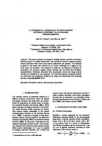
The optimal control law u(t) and the state variable x(t) are computed with m = 4 and 32 for BPFs and m = 4 for SLPs . The results obtained are shown in Figure 1 and 2. It is clear from the figures that the results of BPF approach and SLP approach follow each other. Table 1 shows the J value and computational time for different m values for both for the approaches. It is interesting to note from Table 1 that the computational time of BPF approach with m = 32 is less than what SLP approach has taken with m = 4. It is not surprising as BPFs are all unity, see Equation (1), and therefore we do not have to specifically generate them the way SLPs are generated, and use the same in further computations. This accounts for great saving in computational time. All the computations are done with MATLAB 7 and Pentium 4 CPU 3.00 GHz, 1 GB RAM system.
G0, m −1 ⎤ L G1, m −1 ⎥⎥ if BPFs used (37) M ⎥ ⎥ L Gm −1, m −1 ⎦⎥ L
G11 M Gm −1,1
⎡ ⎢ G00 ⎢ ⎢ ⎢ G = (t f − t0 ) ⎢ 10 ⎢ M ⎢ ⎢ ⎢Gm −1,0 ⎣
G0, m −1 ⎤ ⎥ (2m − 1) ⎥ G1, m −1 ⎥ G11 L ⎥ 3 (2m − 1) ⎥ if SLPs used ⎥ M M ⎥ Gm −1,1 Gm −1, m −1 ⎥ L 3 (2m − 1) ⎥⎦ (38) Consequently Equation (34) can be written as G01 3
L
xˆ = Muˆ + vˆ
where
11 2 2 ∫ ⎡ x (t ) + 2u (t ) ⎤⎦ dt 20⎣
(36)
and ⎡ G00 ⎢ G 10 Gˆ = T ⎢ ⎢ M ⎢ ⎣⎢Gm −1,0
)
(
M = M1 H T ⊗ B
(
(39)
)
(40)
) (
)
M1 = ⎡ I mn − H T ⊗ A − H T ⊗ I n Gˆ ⎤ ⎣ ⎦
−1
(41)
and
17
SANJEEB KUMAR KAR / ELEKTRIKA, 11(1), 2009, 15-18
0.2
BPFs for m = 32 BPFs for m = 4 SLPs for m = 4
0 -0.2
SLP
control
u(t)
-1 -1.2 -1.4
0
0.1
0.2
0.3
0.4
0.5
0.6
0.7
0.8
0.9
BPFs for m = 32 BPFs for m = 4 SLPs for m = 4
REFERENCES [1] Y. A. Kochetkov and V. K. Tomshin, “Optimal control of deterministic systems described by integrodifferential equations,” Automation and Remote Control, vol. 39, no. 1, pp. 1-6, 1978. [2] J. W. Brewer, “Kronecker products and matrix calculus in system theory,” IEEE Trans. Circuits and Systems, vol. CAS-25, no. 9, pp. 772-781, 1978. [3] G. P. Rao, Piecewise Constant Orthogonal Functions and Their Application to Systems and Control, LNCIS, vol. 55, Springer-Verlag, Berlin, 1983. [4] C. Hwang, D. H. Shih and F. C. Kung, “Use of block-pulse functions in the optimal control of deterministic systems,” Int. J. Control, vol. 44, no. 2, pp. 343-349, 1986. [5] D. H. Shih and F. C. Kung, “Optimal control of deterministic systems via shifted Legendre polynonials,” IEEE Trans. Automatic Control, vol. AC-31, no. 5, pp. 451-454, 1986. [6] D. H. Shih and L. F. Wang, “Optimal control of deterministic systems described by integrodifferential equations,” Int. J. Control, vol. 44, no. 6, pp. 1737-1745, 1986. [7] J. H. Chou, “Application of Legendre series to the optimal control of integrodifferential equations,” Int. J. Control, vol. 45, no. 1, pp. 269-277, 1987. [8] K. B. Datta and B. M. Mohan, Orthogonal Functions in Systems and Control, World Scientific, Singapore, 1995.
1.8
state
1.6
x(t) 1.4
1.2
1
0.1
0.2
0.3
1.5032
The author would like to thank Dr. B. M. Mohan, Professor, Department of Electrical Engineering, IITKharagpur, India, for his help and inspiration in this work.
2.2
0
0.8590
ACKNOWLEDGMENT
Figure 1. BPF and SLP solutions of control variables
0.8
4
1
time
2
1.5039
In this paper a unified approach is presented to solve linear quadratic optimal control problem of time-invariant deterministic systems described by integro-differential equations. The proposed approach is computationally simpler than the methods in [1, 4 - 7]. In the example considered, the results obtained with m = 4 SLPs is quite satisfactory. Since BPFs are piecewise constant and the actual solution is smooth, one has to choose a large value for m in BPF approach in order to improve upon the accuracy.
-0.8
-1.6
0.4680
5. CONCLUSION
-0.4 -0.6
32
0.4
0.5
0.6
0.7
0.8
0.9
1
time
Figure 2. BPF and SLP solutions of state variables
Table 1.Computational time and cost function Method
m
Time in sec.
J Value
BPF
4
0.2810
1.5451
8
0.3120
1.5136
16
0.3750
1.5058
24
0.4220
1.5044
18