hardware or software: De nition 3 A BSB, Bi, is de ned as a six-tuple. Bi = < as;i; ts;i; ah;i; th;i; ri; wi > where as;i and ts;i are the area and execution time of.
PACE: A Dynamic Programming Algorithm for Hardware/Software Partitioning Peter Voigt Knudsen and Jan Madsen
Department of Computer Science, Technical University of Denmark, DK-2800 Lyngby, Denmark
Abstract.
This paper presents the PACE partitioning algorithm which is used in the LYCOS co-synthesis system for partitioning control/data ow graphs into hardwareand software parts. The algorithm is a dynamic programming algorithm which solves both the problem of minimizing system execution time with a hardware area constraint and the problem of minimizing hardware area with a system execution time constraint. The target architecture consists of a single microprocessor and a single hardware chip (ASIC, FPGA, etc.) which are connected by a communication channel. The algorithm incorporates a realistic communication model and thus attempts to minimize communication overhead. The time-complexity of the algorithm is O(n2 �A) and the space-complexity is O(n �A) where A is the total area of the hardware chip and n the number of code fragments which may be placed in either hardware or software.
1 Introduction The hardware/software partitioning of a system speci cation onto a target architecture consisting of a single CPU and a single ASIC has been investigated by a number of research groups [2, 5, 1, 7, 8, 11]. This target architecture is relevant in many areas where the performance requirements cannot be met by generalpurpose microprocessors, and where a complete ASIC solution is too costly. Such areas may be found in DSP design, construction of embedded systems, software execution acceleration and hardware emulation and prototyping [10]. One of the major di�erences among partitioning approaches is in the way communication between hardware and software is taken into account during partitioning. Henkel, Ernst et al. [2, 1, 6] present a simulated annealing algorithm which moves chunks of software code (in the following called blocks) to hardware until timing constraints are met. The algorithm accounts for communication and only variables which need to be transferred are actually taken into account, i.e., the possibility of local store is exploited. Gupta and De Micheli [5] present a partitioning approach
which starts from an all-hardware solution. Their algorithm takes communication into account and is able to reduce communication when neighboring vertices are placed together in either software or hardware. The system model presented by Jantsch et al. [7] ignores communication. They present a dynamic programming algorithm based on the Knapsack algorithm which solves the partitioning problem for the case where some blocks include other blocks and are therefore mutually exclusive. The algorithm has exponential memory requirements which makes it impractical to use for large applications. To solve this problem they propose a pre-selection scheme which only selects blocks which induce a speedup greater than 10%. However, this pre-selection scheme may fail to produce good results as communication overhead is ignored. Kalavade and Lee [8] present a partitioning algorithm which does take communication into account by attributing a xed communication time to each pair of blocks. This approach may overestimate the communication overhead as more variables than actually needed are transferred. In this paper we present a dynamic programming algorithm called PACE [9] which solves the hardware/software partitioning problem taking communication overhead into account.
2 System Model This section presents the system model used by the partitioning algorithm, and describes how it is obtained from the functional speci cation.
2.1 The CDFG Format The functional speci cation, which is currently described in VHDL or C, is internally represented as a control/data ow graph (CDFG) which can be de ned as follows: De nition 1 A CDFG is a set of nodes and directed edges (N, E) where an edge ei;j = (ni ; nj ) from ni 2 N to nj 2 N , i 6= j , indicates that nj depends on ni because of data dependencies and/or control dependencies. De nition 2 A node ni 2 N is recursively de ned as ni = DFG j Cond j Loop j FU j Wait
Cond = (Branch1; Branch2) Loop = (Test; Body) Branch1 = CDFG Branch2 = CDFG Test = CDFG Body = CDFG FU = CDFG where a DFG is a pure data ow graph without control structures, FU represents a function call, Wait is used for synchronization with the environment, Branch1 and Branch2 are the CDFGs to be executed in the \true" and \false" branch case of a conditional Cond respectively and Test and Body are the test and body CDFGs of a Loop.
2.2 Derivation of Basic Scheduling Blocks In order to be able to partition the CDFG, it must rst be divided into fragments, in the following called Basic Scheduling Blocks or BSBs. For each node ni in the CDFG, a BSB is created as shown in gure 1. Each MAIN Wait Fu
DFG Body
Test
DFG
Cond Branch1
DFG
Loop
DFG
DFG
CDFG
Branch2
DFG
Wait DFG Loop Test FU DFG Body DFG Cond Branch1 DFG Branch2 DFG DFG BSB hierarchy
Figure 1: The BSB hierarchy and its correspondence with the CDFG. BSB can have child BSBs which are shown indented under the BSB. In this way a BSB hierarchy which re ects the hierarchy of the CDFG is obtained. A BSB stores information which is used by the partitioning algorithm to determine whether it should be placed in hardware or software: De nition 3 A BSB, Bi , is de ned as a six-tuple = where as;i and ts;i are the area and execution time of Bi when placed in software, ah;i and th;i are the area and execution time of Bi when placed in hardware and ri and wi contain the read-set and write-set variables of Bi . Bi
< as;i ; ts;i ; ah;i ; th;i ; ri ; wi >
In order to be able to control the number and sizes of the BSBs which are considered by the partitioning
algorithm, parent BSBs can be collapsed as to appear as single BSBs instead of the child BSBs they are composed of. This is illustrated in gure 2. The partitionWait DFG Loop Test FU DFG Body DFG Cond Branch1 DFG Branch2 DFG DFG
Wait DFG Loop Test FU DFG Body DFG Cond
Wait DFG Loop Test
DFG
DFG
Original Hierarchy. Seven leaf BSBs.
Cond BSB collapsed. Test and Body BSBs Six leaf BSBs. collapsed. Five leaf BSBs.
Body
Figure 2: Adjusting BSB granularity by hierarchical collapsing. ing algorithm only considers leaf BSBs which are BSBs which have no children. The leaf BSBs are marked with a dot in the gure. When BSBs are collapsed, the number of leaf BSBs decreases. As the execution time of the PACE algorithm depends quadratically on the number of BSBs, it is relevant to be able to control the number of BSBs in this way. As all leaf BSBs together make up the total system functionality, we can now de ne the system speci cation in terms of leaf BSBs:
De nition 4 A system speci cation S is described as
an ordered list of n leaf BSBs, i.e. fB1; B2 ; : : : ; Bn g where Bi denotes BSB number i.
In order to estimate performance, it is necessary to know how many times each BSB is executed for typical input data. This information is obtained from pro ling. It is convenient to de ne two global functions which return pro ling information for individual BSBs and individual variables:
De nition 5 The function pc : Bi 2 S ! Nat returns the number of times Bi has been executed in a pro ling run1. De nition 6 Let V denote the set of all variables from the read-sets and write-sets of the BSBs in S . Then, for a given variable v from the read-set or write-set of Bi , the function ac : v 2 V ! Nat returns the number of times the variable is accessed by Bi :2 ( ) ( ) ac( ) = pc( ) v 2 ri
_
v 2 wi
)
v
1 \pc" is short for \pro ling count". 2 \ac" is short for \access count".
Bi
3 Problem formulation The partitioning model which the PACE algorithm uses is illustrated in gure 3. In this model hardware SW
HW
SW
B1
B1
B2
B2
HW
De nition 9 The total (possibly negative) speedup induced by moving a BSB sequence Si;j to hardware is denoted si;j and is computed as si;j =
Xj pc(Bk)(ts;k ? th;k) ? k i X ac(v)ts!h + X ac(v)th!s) ( =
v2wi;j
v2ri;j
B3
B3
S 3,4 B4
B4
ai;j
B6
B6
De nition 10 The area penalty ai;j of moving Si;j to hardware is computed as the sum of the individual BSB areas:
B5
B5
where ts!h and th!s denote the software-to-hardware and hardware-to-software communication times for a single variable, respectively.
=
S 6,7 B7
B7
B8
B8
A)
B)
Figure 3: Partitioning model used by PACE: a) Example of actual data-dependencies between hardwareand software BSBs, b) How data-dependencies between adjacent hardware BSBs and software BSBs are interpreted in the model. BSBs and software BSBs cannot execute in parallel. Furthermore, adjacent hardware BSBs are assumed to be able to communicate the read/write variables they have in common directly between them without involving the software side. As illustrated in the gure, a given hardware/software partition can be thought of as composed of sequences of adjacent BSBs which only communicate their e�ective read- and write-sets from/to the software side. The following de nitions formalize these assumptions.
De nition 7 Si;j , j � i, BSBs fBi ; Bi+1 ; : : : ; Bj g.
denotes the sequence of
De nition 8 The e�ective read-set and the e�ective write-set of a sequence Si;j are denoted ri;j and wi;j respectively and are de ned as ri;j wi;j
= ( = (
+1 [ � � � [ rj ) n (wi [ wi+1 [ � � � [ wj ) +1 [ � � � [ wj ) n (ri [ ri+1 [ � � � [ rj )
r i [ ri
w i [ wi
Using these de nitions and the BSB de nitions given in section 2.2 we can now compute the speedup induced by moving a sequence of BSBs from hardware to software:
X j
k
=i
ak
In section 4.2 we discuss how the e�ect of hardware sharing is taken into account. Note that in calculating the speedup and area of a sequence it is not considered that hardware synthesis may synthesize the sequence as a whole which would probably reduce both sequence area and execution time as compared to just summing the individual area- and execution time components as described above. Incorporating such sequence optimizations in the estimations will be fairly straightforward but has not been carried out yet. Note, however, that the improvement in speedup induced by all BSBs within the sequence being able to communicate directly with each other is taken into account. The partitioning problem can now be formulated as that of nding the combination of non-overlapping hardware sequences which yields the best speedup while having a total area penalty less than or equal to the available hardware area A.
4 Software, Hardware and Communication Estimation This section describes how hardware area- and execution time, software execution time, and communication time are estimated.
4.1 Software Estimation Software execution time for a pure DFG (i.e., no control ow) is estimated by performing a topological sort (linearization) of the nodes in the DFG. The nodes are then translated into a generic instruction set with the addressing modes of the instructions determined by data-dependencies and a greedy register allocation scheme. The execution times of the generic instructions
are then determined from a technology le corresponding to the target microprocessor. This is similar to the approach described in [3], where good estimation results are reported, and the same technology les for the 8086, 80286, 68000 and 68020 microprocessors are used. The execution time of the DFG is obtained by summing the execution times of the generic instructions and multiplying the sum with the pro ling count for the DFG. Execution times for higher level constructs such as loop BSBs and branch BSBs are obtained on basis of the execution times of their child BSBs.
4.2 Hardware area estimation A common way of estimating the hardware area of a BSB is to estimate how much area a full hardware implementation of the BSB will occupy. This includes hardware to execute the calculations of the BSB and hardware to control the sequencing of these calculations. If the total chip area is divided into a datapath area and a controller area, each BSB moved to hardware may be viewed as occupying a part of the datapath and a part of the controller. Figure 4a shows this model when one BSB has been moved to hardware. B1
Controller
Datapath
Area = A C1+ A D1
A)
B2
Controller
Area
Datapath
(A C1+ A C2 ) + (A D1+ A D2 ) B)
B1
Controller
4.3 Hardware execution time estimation The hardware execution time for a DFG is determined by dynamic list based scheduling [4] which attempts to utilize the hardware modules in the given allocation in order to maximize parallelism and thereby minimize execution time. The execution time obtained in this way is multiplied with the pro ling count for the DFG. The execution time for higher level constructs is obtained as in the software case.
4.4 Communication estimation Communication is currently assumed to be memory mapped I/O. The transfer of k variables from software to hardware is assumed to require k generic MOV microprocessor instructions and k Import operations as de ned in the hardware library. Communication from hardware to software is estimated in the same way, just using the hardware Export operation instead.
5 The PACE algorithm
B2
Datapath
Area = (A C1 + A C2) + A
controller, and will depend on the number of timesteps required for executing the BSB. The hardware area of a BSB therefore depends on its execution time.
D
C)
Figure 4: BSB area estimation which accounts for hardware sharing: a) Controller- and datapath area for a single BSB, b) When sharing hardware, the total area for multiple BSBs are less than the summation of the individual areas, c) Variable controller area and xed datapath area for multiple BSBs with hardware sharing. When several BSBs are moved to hardware they may share hardware modules as they execute in mutual exclusion. Hence, an approach which estimates area as the summation of datapath and control areas for all hardware BSBs will probably overestimate the total area. This problem is depicted in gure 4b where the area of the datapath is not equal to the sum of the individual BSB datapaths. In our approach the datapath area is the area of a set of preallocated hardware modules in the datapath as illustrated in gure 4c. The BSBs share these modules and the controller area is the area left for the BSB controllers. The hardware area of a BSB is then estimated as the hardware area of the corresponding
The idea behind the PACE algorithm is best illustrated by an example. Figure 5 shows four BSBs which must be partitioned as to reach the largest speedup on the available area A=3. The speedup and area penalty for a single BSB which is moved to hardware is shown below each BSB. The numbers between two BSBs denote the extra speedup which is incurred because of the BSBs being able to communicate directly with each other when they are both placed in hardware. s BC =2
s AB =2 A
aA = 1 sA = 5
B
aB = 1 sB = 10
s CD =4 C
aC = 1 sC = 2
D
aD = 1 sD = 10
Figure 5: Example of partitioning problem with communication cost considerations. Obviously B and D should be placed in hardware as they have large inherent speedups. This leaves room for one more BSB. Should it be A or C? The answer to this is not obvious as A induces a large inherent speedup but a small communication speedup when placed together with B in hardware, whereas C induces a smaller inherent speedup but on the other hand induces a large communication speedup when placed together with B and D in hardware. The following paragraphs explain how the PACE algorithm solves this problem. The algorithm utilizes the previously mentioned fact, that any possible partition can be thought of as
composed of sequences of BSBs. If A, C and D are chosen for hardware, it corresponds to choosing the sequences SA;A and SC;D . The speedup of sequence SC;D is larger than the sum of speedups of its components C and D due to the extra communication speedup induced by both blocks being chosen for hardware. So a natural approach will be to calculate the areas and speedups of all sequences of BSBs, and chose the combination of sequences that induces the largest speedup. The areas and speedups of all sequences are calculated and shown in table 1. The ordering and grouping of BSBs is explained below. Sequence Elements Area Speedup Group A: All sequences ending with A SA;A A 1 5 Group B: All sequences ending with B SA;B AB 2 SB;B B 1 Group C: All sequences ending with C SA;C ABC 3 SB;C BC 2 SC;C C 1 Group D: All sequences ending with D SA;D ABCD 4 SB;D BCD 3 SC;D CD 2 SD;D D 1
17 10 21 14 2 35 28 16 10
Table 1: Grouping of sequences. The problem is to nd the combination of nonoverlapping sequences which ts the available area A and whose speedup sum is as large as possible. This problem cannot be solved with an ordinary Knapsack Stu�ng algorithm as some of the sequences are mutually exclusive (because they contain identical BSBs) and therefore cannot be moved to hardware at the same time. But if the sequences are ordered and grouped as shown in the table, a dynamic programming algorithm can be constructed which does not attempt to chose mutually exclusive sequences for hardware at the same time. The algorithm works as follows. Assume rst that for each group up to and including group C the best (maximum speedup) combination of sequences has been found and stored for each (integer) area a from zero up to the available area A. Assume then that for instance sequence SC;D with area aC;D is selected for hardware at the available area a. How is the optimal combination of sequences on the remaining area a ? aC;D then found? As C and D have been chosen for hardware, only A and B remain. So the best solution on the remaining area must be found in group B which contains the best combination of sequences for all BSBs from the set fA,Bg. Similarly, if the \sequence" SD;D is chosen for hardware, the best combination on the remaining area is found in group C. The optimal combination is always found in the group whose letter in the alphabet comes immediately before the letter of the rst index in the chosen sequence. The important thing to note is that when a sequence from
Area: 1
2
3
4
Group A: (a=1,s=5)
A
S a,a
5
5
5
5
Best:
S :5 a,a
S :5 a,a
S :5 a,a
S :5 a,a
Group B: AB
(a=2, s=17)
S a,b
17
17
17
B
(a=1. s=10)
S b,b
10
10 + 5 = 15
10 + 5 = 15
10 + 5 = 15
Best:
S : 10 b,b
S : 17 a,b
S : 17 a,b
S : 17 a,b
21
21
Group C: ABC
(a=3, s=21)
S a,c
BC
(a=2, s=14)
S b,c
(a=1, s=2)
S c,c Best:
C
Group D:
14
14 + 5 = 19
14 + 5 = 19
2
2 + 10 = 12
2 + 17 = 19
2 + 17 = 19
S : 10 b,b
S : 17 a,b
S : 21 a,c
S : 21 a,c 35
ABCD
(a=4, s=35)
BCD
(a=3, s=28)
S b,d
CD
(a=2, s=16)
S c,d
D
(a=1, s=10)
S d,d
10
Best:
S
S a,d
b,b
: 10
28
28 + 5 = 33
16
16 + 10 = 26
16 + 17 = 33
10 + 10 = 20
10 + 17 = 27
10 + 21 = 31
S : 20 d,d
S : 28 b,d
S : 35 a,d
, 2] Speedup[S d,d
BestChoice[D, 4] BestSpeedup[D, 4]
Figure 6: The PACE algorithm employed for a simple example. group X has been chosen, the optimal combination of sequences on the remaining area can be found in one of the groups A to pred(X), and, when sequences are selected as above, no mutually exclusive BSBs are selected simultaneously. In this way the best solutions for a given group can always be determined on basis of the best solutions found for the previous groups. Figure 6 shows how the best combination of sequences can be found using three matrices; Speedup[1..nS , 0..A], BestSpeedup[1..n,1..A] and BestChoice[1..n, 0..A]. nS is the number of sequences, n is the number of BSBs and A is the available area. Zero entries are not shown. Arrows indicate where values are copied from, but arrows are not shown for all entries in order to make the gure more readable. The Speedup matrix contains for each sequence and each available area the best speedup that can be achieved if that sequence is rst moved to hardware and then sequences from the previous groups are moved to hardware. In the gure, Speedup[SB;C, 3] is 19 and is found as the inherent speedup of SB;C which is 14 plus the best obtainable speedup 5 on area 3 ? aB;C = 3 ? 2 = 1 in group A (as B and C have been chosen). The BestSpeedup matrix contains for each group (which there are n of) and each area the best speedup that can be achieved by rst selecting a sequence from that group or one of the previous groups. It can be calculated as BestSpeedup[g ,
]=
a
max (max (Speedup[ 2 S
g
S
,a]); BestSpeedup[pred(g ),a] )
The BestChoice[g,a] matrix identi es the choice of sequence that gave this maximum value. The last two matrices are interleaved and typeset with bold letters in the gure. In the example, BestChoice[C, 3] is 21 as this is the maximum speedup that can be found in group C with available area 3 and it is larger than the largest speedup that could be found in the previous groups, namely 17. The corresponding choice of sequence is SA;C . In contrast, BestSpeedup[C,1] and BestChoice[D,1] are copied from the corresponding entries of the previous group. For group C this is because all Speedup entries in that group for area 1 are smaller than the best speedup 10 achieved with only sequences from groups up to and including B. For group D, Speedup[SD;D, 1] is also 10, so the choice of best sequence for this group is arbitrary. The solution to the posed problem is found in the BestChoice[D, 3] and BestSpeedup[D,3] entries. The best initial choice is sequence SB;D with the corresponding total speedup of 28. As the area of this sequence is 3, no other sequences were taken, and need thus not be found by backtracking. This shows that it was best to chose C for hardware instead of A. The area 4 was included in the gure to show that the algorithm correctly chooses all four BSBs for hardware when there is room for them. This can be seen from the [D,4] entries. Once the BestSpeedup and BestChoice lines have been calculated for each group, the Speedup values are no longer needed. Actually, the Speedup matrix is not needed at all, as it can be replaced by the BestSpeedup matrix whose maximum values can be calculated \on the run". This is because we are only interested in maximum values and corresponding choice of sequences for each group. This means that instead of the memory requirements being proportional to the number of sequences nS , they are now proportional to n, as only the BestSpeedup and BestChoice matrices are needed. The PACE algorithm is shown as algorithm 1. After the algorithm has been run, the best speedup that can be obtained is found in the entry BestSpeedup[NumBSBs, AvailableArea]. But as for the simple Knapsack algorithm, reconstruction of the chosen sequences and thereby of the chosen BSBs is necessary.
5.1 Algorithm Analysis Direct inspection of the PACE algorithm shows that the time complexity is O(n2 � A) and the space complexity is O(n � A) (the PACE-reconstruct algorithm obviously has smaller time and area complexity and can hence be disregarded). Note that areas must be expressed as integral values. A can be reduced (at the expense of partitioning quality) by using a larger \area granularity", for example by expressing BSBs sizes in
PACE (n; A) �
f
for all groups g = 1 to n do for all areas a = 0 to A do f BC[g,a] fg; BS[g,a] 0; g g for all groups g = 1 to n do f HighBSB g; for LowBSB = 1 to HighBSB do f
SeqArea area(SLowBSB;HighBSB ); SeqSpeedup speedup(SLowBSB;HighBSB ); for all areas a = SeqArea to A do f if (LowBSB = 1) then f if SeqSpeedup > BS[g, a] then f BS[g,a] SeqSpeedup; BC[g,a] SLowBSB;HighBSB ;
g g else f if SeqSpeedup + BS[LowBSB-1, a-SeqArea] > BS[g, a] then f g
g
BS[g,a] SeqSpeedup + BS[LowBSB-1, a-SeqArea]; BC[g,a] SLowBSB;HighBSB ;
g g if (HighBSB > 1) for all areas a = 0 to A do if BS[g-1, a] > BS[g, a] then f g g
g
BS[g, a] BC[g, a]
BS[g-1, a]; BC[g-1, a];
return BC[]; return BS[];
PACE-reconstruct (n; A; BS []; BC []) �
f
g
HwBSBList fg; AStart 0; Found false; while (AStart