Paper Visual Instance Retrieval with Deep Convolutional ... - J-Stage

ITE Trans. on MTA Vol. 4, No. 3, pp. 251-258 (2016)

Copyright © 2016 by ITE Transactions on Media Technology and Applications (MTA)

Paper Visual Instance Retrieval with Deep Convolutional Networks Ali S. Razavian † , Josephine Sullivan † , Stefan Carlsson † , Atsuto Maki † Abstract This paper provides an extensive study on the availability of image representations based on convolutional networks (ConvNets) for the task of visual instance retrieval. Besides the choice of convolutional layers, we present an efficient pipeline exploiting multi-scale schemes to extract local features, in particular, by taking geometric invariance into explicit account, i.e. positions, scales and spatial consistency. In our experiments using five standard image retrieval datasets, we demonstrate that generic ConvNet image representations can outperform other state-of-the-art methods if they are extracted appropriately.

Key words: Convolutional network, Visual instance retrieval, Multi-resolution search, Learning representation

1. Introduction Visual instance retrieval is amongst widely studied applications of computer vision, and the research progress has been reported based on several benchmark datasets. Using a database of reference images each having a label corresponding to the particular object or scene and given a new unlabeled query image, the task is to find images containing the same object or scene as in the query. Not to mention the accuracy of the retrieval results, there is also the challenge of search efficiency because modern image collections can contain millions if not billions of images. To solve the problem, one has two major design choices: image representations and similarity measures (or distance metrics). The task can be therefore viewed as encoding a large dictionary of image appearances where each visual instance needs a compact but descriptive representation. Image representations based on convolutional networks (ConvNets) are increasingly permeating in many established application domains of computer vision. Much recent work has illuminated the field on how to design and train ConvNets to maximize performance1) 5) and also how to exploit learned ConvNet representations to solve visual recognition tasks7) 9)11) in the sense of transfer learning. Based on these findings, although less explored, recent works also suggest the potential of ConvNet representations for the task of image retrieval11)13)14) , which we concern ourselves in this paper. Possible alternatives for such a representation include holistic representations where the whole image is mapped to a single vector13)14) and multi-scale schemes where local

Fig. 1

In visual instance retrieval, items of interest often appear in different viewpoints, lightings, scales and locations. The primary objective of the paper is to introduce a generic pipeline that can well handle all those variations.

features are extracted at multiple scale levels11)16) . An essential requirement is that a proper representation should be ideally robust against variations such as scale and position of items in the image. That is, representations for the same instance in different viewpoints, or in various sizes, should be as close to each other as possible. Considering the geometric invariance as our priority, in this paper, we study the multi-scale scheme and design our pipeline including the similarity measure accordingly. Another practical aspect to consider for instance retrieval is the dimensionality and memory requirements of the image representation. Usually, two separate categories are considered; the small footprint representations are encoding each image with less than 1kbytes and the medium footprint representations which have dimensionality between 10k and 100k. The former is required when the number of images is huge and memory is a bottleneck, while the latter is more useful when the number of images is less than 50k. To the best of our knowledge,this work is the first to show that the ConvNet representations are well suited for the task of both

Received December 21, 2015;; Revised Revised March 17, 2016; Accepted April Received ; Accepted 22, 2016 † Royal Institute of Technology (KTH) (Stockholm, Sweden)

251

ITE Trans. on MTA Vol. 4, No. 3 (2016)

small and medium footprint retrieval while our main focus will be on the medium footprint representations. The overall objective of this work is to highlight the potential of ConvNets image representations for the task of visual instance retrieval while taking into account above mentioned factors, i.e. geometric invariance, the choice of layers, and search efficiency. In sum, the contributions of the paper are three-fold: •

•

•

mise between performance and the representation size. The challenge of this task is to encode the most distinctive representation on small-footprint representations. Depending on the task, the size of representation can vary from 1k dimension to less than 16 bytes 26)32) . The current paper is most related to11)13)14)16) concerning the usage of ConvNet representations. The work in13)14) for instance examined ConvNet representations taken from different layers of the network while focusing on holistic features. The representation in the first fully connected layer was the choice in11) , and it was also concluded13) to perform the best but still not better than other state-of-the-art holistic features (e.g. Fisher vectors30) ). It is a natural next challenge to improve further the performance to the extent comparable to or better than the state-of-the-art approaches by taking different aspects of representations and similarity measures into consideration.

We demonstrate that a ConvNet image representation can outperform state-of-the-art methods on all the five standard retrieval datasets if they are extracted suitably. These datasets cover the whole spectrum of patterns from texture-less to repeated ones. We formulate a powerful pipeline for retrieval tasks by extracting local features based on ConvNet representations. We suggest and show that spatial pooling is well suited to the task of instance retrieval regarding dimensionality reduction and preserving spatial consistency.

3. The ConvNet representation of an image We first review our design choices as regards to the ConvNet representation we obtain from a deep convolutional network, preceding the description of our general pipeline which is provided in the next section. The basic idea underlying our pipeline is that we have a way to extract a good feature representation of the input, I, whether it is an image or its sub-patch. Such a representation can be defined by exploiting generic ConvNets trained on ImageNet. 3. 1 The choice of layer: the final convolution layer In the following, we employ the standard architecture for the convolutional network21) consisting of multiple convolutional layers, Layerj (I)(j = 1, ..., c), and three fully connected layers. Now, let us visit possible interpretation on the function that each layer has4) : units in the first convolutional layer respond to simple patterns like edges or textures. Second layer’s units aggregate those responses into more complex patterns. As the process continues further (deeper), units are expected to respond to more and more complex patterns in their corresponding receptive fields4)31) . The first fully connected layer has pooled all the patterns together and the next two fully connected layers learn a non-linear classifier and estimate the probability of each class. Nevertheless, the ability to recognize specific patterns should be an integral component of an image retrieval system. Given this, it makes more sense to use the responses of the last convolutional layer (Layerc (I)) each response in this layer corresponds to a specific appearance pattern (up to the deformations allowed by the max-pooling and activation function applied after each convolutional layer) occurring in

It should also be noted that our pipeline does not rely on the bias of the dataset as it heavily relies on the generic ConvNet train on ImageNet (except to estimate the distribution of the data for the representation). Therefore, it can be highly parallelized. For a fair comparison, the benchmarking of our methods will be with pipelines that do not include any search refinement procedures such as query expansion17) and spatial re-ranking18)19) .

2. Related work It was not until Krizhevsky and Hinton20) evaluated their binary codes that representations produced by deep learning were considered for image retrieval. Since the recent success of deep convolutional networks on image classification21) , trained with large scale datasets22) , the learned representations of ConvNet attracted increasing attention also for other applications of visual recognition. See for example4)5)7)8) . Among those a few papers have recently shown promising early results for image retrieval tasks11)13)14)23) using ConvNet representations although the subject is yet to be explored. The key factor for the task of visual instance retrieval is to find an efficient image representation. Popular approaches for this goal include vector aggregation methods such as the bag-of-words (BOW) representation24) , the Fisher Vector (FV)25) , and the VLAD representation26) . The performance of27) and28) have been among the state-of-the-art in this domain. Another line of work in retrieval deals with the compro252

Paper » Visual Instance Retrieval with Deep Convolutional Networks

0.5

Fig. 2

Performance

0.4

Schematic of spatial pooling. The sketches show how the dimensionality of the representation of a convolutional layer can be reduced by max-pooling (left:1×1

0.3 0.2 0.1

pooling, right: 2×2 pooling). The width of the volumes corresponds to the number of filters used for con-

Oxford5K(conv) Sculpture6k(conv) Oxford5k(fc) Sculpture6k(fc)

volutions. A 1×1 pooling results in one number per

200

feature map while 2×2 pooling results in four num-

300

400

500

600

700

800

Input image side length

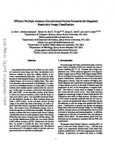
bers. See section 3. 2 for the details. Fig. 3

The effect of rescaling the input image and the choice of layer on retrieval task. Distinctive pat-

a specific large sub-patch of the original image. In fact, experimental evidence is provided in the study for the factors of transferability5) that the last convolutional layer is the best alternative for instance retrieval. Our intuition is that, at this level, relevant information for instance retrieval that is not suited for classification is still preserved. Another benefit of using Layerc (I) is that it enables us to extract local features for rectangular patches which is an important advantage for retrieval. This is in contrast to the case of using a fully connected layer where one would need to either crop a part of the image; this will cause some loss of information or break the aspect ratio, which is harmful to the task of visual retrieval. With these motivations, we use the response maps from Layerc (I), the last convolutional layer in this paper. See Figure 3 for the empirical justifications. 3. 2 Spatial max-pooling As we use a deep and wide network, the dimensionality of this representation is also very large (approximately 40×40×512). It is neither feasible nor practical to compute distances and similarities with vectors of this size. Therefore some form of dimensionality reduction is necessary. We reduce the dimension of our feature vector by exploiting the usual max-pooling applied in the convolutional layers of a ConvNet. The difference is that we have a fixed number of cells in our spatial grid as opposed to a spatial grid of cells of a fixed size. This type of pooling is not new and has been employed before. Because max-pooling as such allows one to input images of variable size into the ConvNet and still extract a fixed sized response before the first fully connected layer. Our experiments confirm that such a low-dimensional representation is more distinctive than the hand-crafted representation of the same memory footprint. Refer to section 5 for details. If we apply spatial pooling with a grid of size 2×2 to

terns for building landmarks are usually small details and by increasing the size of image, the performance on Oxford5k dataset increases while the most distinctive patterns for sculptures are the general shape of them and when the shape of sculpture becomes bigger than the size of the receptive fields, the performance starts to degrade. In our experiments, given the bias of datasets, we found that 600×600 is a reasonable size for our target dataset. See section 5.1 for detailed discussion. Also, Convolutional layers preserve more spatial information which is crucial to the task of retrieval. This observation solidifies the reported experiments of5) . Please refer to section 3.1 for more details.

the original (w×h×512) volume of response maps, we get a 2×2×512 (=2048) dimensional feature vector. Likewise, with a grid of size 1×1, we get a 1×1×512 (= 512) dimensional feature vector. See Figure 2. Max-pooling with a grid of size 2×2 preserves more spatial consistency than 1×1, which is useful for the task of retrieval. But max-pooling over a grid with too many cells generally tends to reduce performance. In this paper, we also exploit the max-pooling to allow us to input larger sized images to the ConvNet than were used while training the original network. Spatial maxpooling is most useful when spatial consistency is the most distinctive feature. 3. 3 Image scale As discussed earlier, the units in convolutional layers respond to patterns in their receptive fields. Therefore, rescaling the size of input image naturally results in a change in the activation of units in the response map. Figure 3 illustrates scaling effect on the performance followed by the explanation in section 5. 1. 253

ITE Trans. on MTA Vol. 4, No. 3 (2016)

a) Multi-resolution Search

None 2×2 3×3

1 Rep. Similarity

1 Rep. Similarity

b) Jittering None 2×2 3×3 4×4

0.8

0.6

0.4

0.8

0.6

Fig. 5

0.4 10−0.3 100 100.3 100.6 Reference to query scale

100.9

10−0.3 100 100.3 100.6 Reference to query scale

c) Multi-resolution Search

Schematic of distance matrix between two images: The distance between two images is computed by

100.9

pooling the distances between different patches of the

d) Jittering

query and the reference image according to equations 1 Rep. Similarity

Rep. Similarity

1

0.8

0.6

None 2×2 3×3 4×4

0.4 0

0.2

0.4

0.6

Overlap ratio

Fig. 4

0.8

(3-4).

0.8

0.6

1

cations. In fact, we extract patches of L different sizes. The different lengths of the side of the patches are   2w 2h , hl = s = max wl = , for l = 1, . . . , L l+1 l+1 (1)

None 2×2 3×3

0.4 0

0.2

0.4

0.6

0.8

1

Overlap ratio

The effect of Multi-resolution search and Jittering on patch similarities: a) Multi-resolution search is helpful when the item of interest has appeared on a smaller scale in the reference image than the query image. b) Jittering provides more robust results and is helpful in particular when the item of interest has appeared on a bigger scale in the reference image than the query. c & d) Both Multi-resolution search and Jittering are helpful when the overlap between the query image and the reference image decreases. Please refer to 4 for discussions.

For each square sub-patch of size s, we extract l2 subpatches centered at the locations   wl hl + (i − 1) bw , + (j − 1) bh , (2) 2 2 w − wl h − hl , and bh = , (l = | 1) where bw = l−1 l−1 for i = 1, . . . , l and j = 1, . . . , l. If the boundary of the square sub-patch exceeds the boundary of the image, we crop the rectangular sub-patch that is within the valid portion of the image. Finally, we resize all the sub-patches to have the same area and then extract its ConvNet representation. We should mention that we want all the sub-patches to have the same bias and in the ideal case, all the patches should have the same aspect ratio. To achieve this, we try to extract square sub-patches wherever possible and only extract rectangular sub-patches when there is no other option. In our experiments, we set L = 4 and therefore extract 4 30(= l=1 l2 ) sub-patches from each image. Multi-resolution search is most helpful when the item of interest has appeared on a smaller scale at an arbitrary position in the reference image. For the justification on why extracting local patches from each image works for the task of instance retrieval, please refer to the recent work of33) . Jittering It is known that jittering increases the performance of ConvNet representations21) . That is, to have a more robust pipeline, instead of employing one patch from the query, we extract multiple patches in the same manner that we extracted sub-patches from reference images. Jittering is a powerful technique when the item of interest has appeared partially or in a bigger scale in the reference image.

It should be noted that max-pooling operation needs be consistent across all the patches to provide meaningful comparisons and therefore all the images should be rescaled to have the same area.

4. Pipeline for measuring similarities of images In this section, we describe our general pipeline exploiting multi-resolution search and approach to compute the distance (similarity) between a query and a reference image. The items of interest (objects, buildings, etc.) in the reference and query images can occur at any location and scale. Then, different scales and other variations of input images may affect the behavior of convolutional layers as images pass through. Facing with this potential issues, we choose to perform a form of multi-scale spatial search when we compute the distance (similarity) between a query image and a reference image. Our search has two distinct sets of parameters and definitions: the first set describes the number, size and location of the sub-patches we extract from each query and reference images I. The second set defines how we use the sub-patches extracted from both the query image and the reference image to compute the distance between the two images. We now describe the two steps in more detail. 4. 1 Extracting local features Multi-resolution search From each reference image, we extract multiple sub-patches of different sizes at different lo254

Paper » Visual Instance Retrieval with Deep Convolutional Networks

Method

#dim Oxford5k Paris6k Holidays Sculp6k UKB

Method

#dim Oxford5k Paris6k Sculp6k Holidays UKB Ox105k

Baseline

512

46.2

67.4

74.6

46.5

90.6

MR2×2 MR3×3 MR4×4

2.5k 7k 15k

58.0 63.4 65.5

68.0 68.5 68.5

70.7 70.2 69.1

40.3 39.8 39.5

85.9 77.5 65.8

Max pooling + l1 dist. Max pooling(quantized) +l2 dist.

256 32B

53.3 43.6

67.0 54.9

37.7 26.1

71.6 57.8

84.2 69.3

48.9 38.0

MR4×4 + Jtr2×2 MR4×4 + Jtr3×3

15k 15k

71.6 72.4

76.3 77.8

78.5 82.2

40.1 38.9

88.0 92.7

VLAD+CSurf15) mVLAD+Surf15) T-embedding30) T-embedding30)

128 128 128 256

29.3 38.7 43.3 47.2

-

-

73.8 71.8 61.7 65.7

83.0 87.5 85.0 86.3

35.3 40.8

MR4×4 + PCAw MR4×4 + Jtr2×2 + PCAw MR4×4 + Jtr3×3 + PCAw

8k 8k 8k

73.0 80.7 82.4

71.0 82.3 86.0

74.7 85.6 89.5

36.1 43.2 46.3

84.2 93.8 95.8

Sum pooling + PCAw29) Ng et al,23)

256 128

58.9 59.3

59.0

-

80.2 83.6

91.3 -

57.8 -

MR4×4 + Jtr3×3 + SP2×2 + PCAw

32k

84.3

87.9

89.6

59.3

95.1

The top two rows show our results. ConvNet based

51.4 82.5 83.8

81.0 80.5

82.7 88.0

45.4 -

90.5 -

methods constantly outperform previous s.o.a. for

BoB 35) CVLAD 38) PR-proj 27) ASMK+MA 28)

Table 1

Table 2

Performance of small memory footprint regimes.

small memory footprint representations. Two bottom results refer to the recent advancement in ConvNet

The effect of individual components in our

based instance retrieval methods. For this experi-

pipeline. Baseline refers to computing a single rep-

ment we trained our network similar to OxfordNet

resentation with 1 × 1 spatial pooling. MR refers

but with 256 kernels in the last convolutional layer.

to Multi-resolution search on the reference image

The result reported on Sculpture dataset was com-

where MR2×2 stands for the settings of L = 2, and

puted on 227 × 227 images.

likewise Jtr refers to Jittering on the query image. PCAw refers to PCA whitening and SP refers to spatial pooling.

step and prior to computing the distance between imagepatches. First the representation is L2 normalized. Then given a reference set of training images (X) from the dataset, T a covariance matrix C is calculated (C = (X−μX )n(X−μX ) where n is the size of the reference set) to allow PCA whitening of the data such that a dimensionality reduction of the representation is enabled. We chose to reduce the dimensionality by half.

Evaluation To study the effectiveness of Multi-resolution search and Jittering, we evaluated these two methods on the similarity of 100 random patches extracted from Affine Covariant Regions Dataset10) . We isolated scaling from translation. See Figure 4 for the evaluation results. 4. 2 The distance between query and reference Next, we describe how we measure the distance (similarity) between a query image I (q) and a reference image I (r) . The reference image I (r) generates sets of feature vectors (r) (q) {fi,j,l }. We define the distance between a sub-patch, I∗ , extracted from I (q) and the image I (r) as:   (q) (q) (r) d∗ (I∗ , I (r) ) = min d f∗ , fr,s,m (3)

5. Results We report results on five standard image retrieval datasets: Oxford5k buildings18) , Paris6k buildings34) , Sculptures6k 35) , Holidays36) and UKbench37) . 5. 1 Medium footprint representation & choice of parameters To evaluate our model we used the publicly available network of39) . This network contains 16 convolutional layers followed by three fully connected layers. We should note that we extended the bounding box of query images by half the size of the receptive fields so that the center of receptive fields for all the units remains inside the bounding box. We have earlier displayed in Figure 3 the effect of resizing the input image size on the final result on two datasets. The most interesting jump in performance due to increasing the size of the input image is seen for the Oxford5k building dataset. An explanation for this is as follows. The distinctive elements of the images in the Oxford5k building dataset correspond to relatively small sub-patches in the original image. A response in the last convolutional layer, Lc (I), corresponds to a whether a particular pattern is present in a particular sub-patch of the input image. Increasing the size of the input image means that the area of this sub-patch is a smaller

1< = m< =L, 1< =r,s< =m

where d(·, ·) corresponds to a distance measure between two vectors. Typically d(·, ·) used in equation (3) is the L2 normalized distance.∗ The final distance between I (q) and I (r) is defined by the sum of each query sub-patch’s minimum distance to the reference image: D(I (q) , I (r) ) =

l  l L  

(q)

d∗ (Ii,j,l , I (r) )

(4)

l=1 i=1 j=1

Where d∗ is defined in equation 3. See Figure 5 for a schematic of computing the distance. 4. 3 Post-processing - PCA whitening There are some further optional, but standard postprocessing steps that can be applied after the max-pooling ∗

When d(·, ·) represents a similarity measure, we replace the minimum in equation (3) with a maximum.

255

ITE Trans. on MTA Vol. 4, No. 3 (2016)

Fig. 6

Visualization of relevant images with lowest score.

Fig. 7

Visualization of irrelevant images with highest

For query image (leftmost), four relevant images with

score. For query image (leftmost), four irrelevant im-

the lowest similarity score have been retrieved. As ex-

ages with the highest similarity score have been re-

pected, some portion of these images contain the item

trieved. In some cases, it is even hard for humans to

of interest with the most radical viewpoint or lighting

tell the difference apart.

changes.

useful. Spatial pooling (SP) preserves spatial consistency, and it is always helpful as anticipated when the spatial position of patterns are the most distinctive feature. For example, it boosts the performance for Sculpture dataset where the boundary of the sculpture is the primary source of information. As a whole, the ConvNet representation with the proposed pipeline outperforms all the state-of-the-art on all datasets. None of the numbers reported in this table considers the effect of post-processing techniques such as query expansion or re-ranking which can be commonly applied to different techniques including ours. Figure 6 shows the relevant images in reference set with lowest score for every query. Figure 7 displays irrelevant images with highest score to each query. 5. 2 Small footprint representations In Table 2 we report results for our small memory representations and compare them to those by state-of-the-art methods with 128 or more dimensions. For the ConvNet methods, we can aggressively quantize the encoding of the numbers in each dimension of the representation to reduce the memory use. Preceded by the initial introduction of our proposed pipeline in 20146) , a few authors have advanced the performance of the small footprint retrieval pipelines with ConvNet. Ng et al.23) replaced max pooling with traditional VLAD over the response map. Babenko and Lempitsky29) suggested that sum-pooling can perform better than maxpooling and Arandjelovic et al.12) included learning in the pipeline as opposed to the off-the-shelf usage. Note that

proportion of the area of the input image, i.e. the representation is better at describing local structures. In contrast, increasing the resizing factor on the input image decreases the performance on the Sculpture6k dataset because for these images better recognition seems to be achieved by describing the global structure. For all the experiments, we resized the images to have an area of 600×600 pixels as it turns out to be a good dimension given these datasets. In Table 1 we report results for our medium sized representations and compare their performance to that of other s.o.a. image representations. From examining the numbers one can see that our image retrieval pipeline based on ConvNet representations outperform hand-crafted image representations, such as VLAD and IFV, which mostly require additional iterations of learning from specialized training data. Table 1 shows the results and the effect of each step in the pipeline. Baseline refers to computing a single representation with 1 × 1 spatial pooling. It is evident that reported performance is relatively good already at this stage. Multiresolution search (MR) helps the most in cases when the query item has appeared on a smaller scale in the reference image. The improvement is most noticeable in Oxford5k and Paris6k datasets where each query contains a full size landmark while in the reference set they have appeared in an arbitrary position and scale. On the other hand, employing MR alone degrades the performance on UKB dataset where items have appeared more or less at a uniform scale. Jittering (Jtr) and PCA whitening (PCAw) are almost always 256

Paper » Visual Instance Retrieval with Deep Convolutional Networks

those have been built on the basis of our pipeline which is formulated in the current paper. 5. 3 Memory and computational overhead The memory footprint and computational complexity of our pipeline is in the order of O(L3 ), and therefore, it is important to keep the L small. In our experiments, we only extended L to 4 and the memory footprint corresponding to the last row of Table 1 is 32k for reference images and 16k for query images. The sub-patch distance matrix has around 120M elements for the task of Oxford5k and 350M elements for Holidays and the whole pipeline can fit in the RAM of an average computer. Computing the distance matrix from sub-patch distance matrix according to equations (3-4) takes 30 − 40 seconds on a single CPU core and 50 − 60 milliseconds on a single K40 GPU in our experiment for the task of Oxford5k. This yields to a reasonable time complexity. All the modules in our pipeline can significantly benefit from parallelism. To accelerate the feature extraction process, instead of extracting 30 representations for 30 sub-patches of an image, we feed the image in four different scales and extract the representation from response maps of the last Convolutional layer corresponding to the sub-patches as mentioned earlier.

ment techniques. References 1) Karen Simonyan, Andrea Vedaldi, and Andrew Zisserman, “Deep inside convolutional networks: Visualising image classification models and saliency maps.,” arXiv:1312.6034 [cs.CV], 2013. 2) Ross B. Girshick, Forrest N. Iandola, Trevor Darrell, and Jitendra Malik, “Deformable part models are convolutional neural networks,” arXiv:1409.5403 [cs.CV], 2014. 3) Ken Chatfield, Karen Simonyan, Andrea Vedaldi, and Andrew Zisserman, “Return of the devil in the details: Delving deep into convolutional nets,” arXiv:1405.3531 [cs.CV], 2014. 4) Matthew D. Zeiler and Rob Fergus, “Visualizing and understanding convolutional networks,” in ECCV, 2014, pp. 818–833. 5) Hossein Azizpour, Ali S. Razavian, Josephine Sullivan, Atsuto Maki, and Stefan Carlsson, “Factors of transferability for a generic ConvNet representation,” IEEE Transactions on Pattern Analysis and Machine Intelligence, 2016. 6) Ali S. Razavian, Josephine Sullivan, Atsuto Maki, and Stefan Carlsson, “Visual instance retrieval with deep convolutional networks,” arxiv:1412.6574 [cs.CV], 2014. 7) Maxime Oquab, L´eon Bottou, Ivan Laptev, and Josef Sivic, “Learning and transferring mid-level image representations using convolutional neural networks,” in CVPR, 2014. 8) Jeff Donahue, Yangqing Jia, Oriol Vinyals, Judy Hoffman, Ning Zhang, Eric Tzeng, and Trevor Darrell, “Decaf: A deep convolutional activation feature for generic visual recognition,” in ICML, 2014. 9) Philipp Fischer, Alexey Dosovitskiy, and Thomas Brox, “Descriptor matching with convolutional neural networks: a comparison to SIFT,” arXiv:1405.5769 [cs.CV], 2014. 10) Krystian Mikolajczyk and Cordelia Schmid, “A Performance Evaluation of Local Descriptors,” IEEE Transactions on Pattern Analysis and Machine Intelligence, 2005. 11) Ali S. Razavian, Hossein Azizpour, Josephine Sullivan, and Stefan Carlsson, “CNN features off-the-shelf: an astounding baseline for recognition,” CVPRW, 2014. 12) Relja Arandjelovic, Petr Gronat, Akihiko Torii, Tomas Pajdla, and Josef Sivic, “NetVLAD: CNN architecture for weakly supervised place recognition,” arxiv:1511.07247 [cs.CV], 2015. 13) Artem Babenko, Anton Slesarev, Alexander Chigorin, and Victor S. Lempitsky, “Neural codes for image retrieval,” in ECCV, 2014. 14) Ji Wan, Dayong Wang, Steven Chu Hong Hoi, Pengcheng Wu, Jianke Zhu, Yongdong Zhang, and Jintao Li, “Deep learning for content-based image retrieval: A comprehensive study,” in ACM Multimedia, 2014, pp. 157–166. 15) Eleftherios Spyromitros-Xioufis, Symeon Papadopoulos, Ioannis (Yiannis) Kompatsiaris, Grigorios Tsoumakas, and Ioannis Vlahavas, “A Comprehensive Study Over VLAD and Product Quantization in Large-Scale Image Retrieval,” in IEEE Transactions on Multimedia, 2014, pp. 1713–1728. 16) Yunchao Gong, Liwei Wang, Ruiqi Guo, and Svetlana Lazebnik, “Multi-scale orderless pooling of deep convolutional activation features,” in ECCV, 2014, pp. 392–407. 17) Ondrej Chum, James Philbin, Josef Sivic, Micheal Isard, and Andrew Zisserman, “Total recall: Automatic query expansion with a generative feature model for object retrieval,” in ICCV, 2007. 18) James Philbin, Ondrej Chum, Michael Isard, Josef Sivic, and Andrew Zisserman, “Object retrieval with large vocabularies and fast spatial matching,” in CVPR, 2007. 19) Michal Perdoch, Ondrej Chum, and Jiri Matas, “Efficient representation of local geometry for large scale object retrieval,” in CVPR, 2009. 20) Alex Krizhevsky and Geoffrey E. Hinton, “Using very deep autoencoders for content-based image retrieval,” in Proceedings of the European Symposium of Artifical Neural Networks (ESANN), 2011. 21) Alex Krizhevsky, Ilya Sutskever, and Geoffrey E. Hinton, “ImageNet classification with deep convolutional neural networks,” in NIPS, 2012. 22) J. Deng, W. Dong, R. Socher, L.-J. Li, K. Li, and L. Fei-Fei, “ImageNet: A Large-Scale Hierarchical Image Database,” in CVPR, 2009. 23) Joe Yue-Hei Ng, Fan Yang, and Larry S. Davis, “Exploiting local features from deep networks for image retrieval,” CVPRW, 2015. 24) Josef Sivic and Andrew Zisserman, “Video google: A text retrieval approach to object matching in videos,” in ICCV, 2003. 25) Florent Perronnin and Christopher R. Dance, “Fisher kernels on visual vocabularies for image categorization,” in CVPR, 2007. 26) Herv´e J´egou, Florent Perronnin, Matthijs Douze, Jorge S´anchez, Patrick P´erez, and Cordelia Schmid, “Aggregating local image descriptors into compact codes,” IEEE Transactions on Pattern Analysis and Machine Intelligence, vol. 34, no. 9, pp. 1704–1716, 2012. 27) Karen Simonyan, Andrea Vedaldi, and Andrew Zisserman, “Learning local feature descriptors using convex optimisation,” IEEE Transactions on Pattern Anal-

6. Conclusion We have presented an efficient pipeline for visual instance retrieval based on ConvNets image representations. Our approach benefits from multi-scale scheme to extract local features that take geometric invariance into explicit account. For the representation, we chose to use last convolutional layer while adapting max-pooling, which not only made the layer available in terms of its dimensionality but helped to boost the performance. Throughout the experiments with five standard image retrieval datasets, we demonstrated that generic ConvNet image representations can outperform other state-of-the-art methods in all the tested cases if they are extracted appropriately. Our pipeline does not rely on the bias of the dataset, and the only recourse we make to specialized training data is in the PCA whitening. For our future work, we plan to investigate domain adaptation to improve further the performance. For example, fine-tuning the ConvNet with landmark dataset13) increases the performance on Oxford5k up to 85.3. We would like to highlight that our result should still be viewed as a baseline. Simple additions such as concatenating multi-scale, multilayer and different architecture representations give a boost in performance (e.g. 87.2 for Oxford5k). From our measure of similarity, a rough bound can also be estimated within our framework, which may be useful for a novel search refine257

ITE Trans. on MTA Vol. 4, No. 3 (2016)

ysis and Machine Intelligence, vol. 36, no. 8, pp. 1573–1585, 2014. 28) Giorgos Tolias, Yannis S. Avrithis, and Herv´e J´egou, “To aggregate or not to aggregate: Selective match kernels for image search,” in ICCV, 2013. 29) Artem Babenko, and Victor Lempitsky, “Aggregating Local Deep Features for Image Retrieval” in ICCV, 2015. 30) Herv´e J´egou and Andrew Zisserman, “Triangulation embedding and democratic aggregation for image search,” in CVPR, 2014. ` 31) Bolei Zhou, Aditya Khosla, Agata Lapedriza, Aude Oliva, and Antonio Torralba, “Object detectors emerge in deep scene cnns,” in ICLR, 2015. 32) Antonio Torralba, Rob Fergus, and Yair Weiss, “Small codes and large image databases for recognition” in CVPR, 2008. 33) Ran Tao, Efstratios Gavves, Cees G. M. Snoek, and Arnold W. M. Smeulders, “Locality in generic instance search from one example,” in CVPR, 2014, pp. 2099–2106. 34) James Philbin, Ondrej Chum, Michael Isard, Josef Sivic, and Andrew Zisserman, “Lost in quantization: Improving particular object retrieval in large scale image databases,” in CVPR, 2008. 35) Relja Arandjelovi´c and Andrew Zisserman, “Smooth object retrieval using a bag of boundaries,” in ICCV, 2011. 36) Herv´e J´egou, Matthijs Douze, and Cordelia Schmid, “Hamming embedding and weak geometric consistency for large scale image search,” in ECCV, 2008. 37) David Nist´er and Henrik Stew´enius, “Scalable recognition with a vocabulary tree,” in CVPR, 2006. 38) Wan-Lei Zhao, Herv´e J´egou, Guillaume Gravier, et al., “Oriented pooling for dense and non-dense rotation-invariant features,” in BMVC, 2013. 39) Karen Simonyan and Andrew Zisserman, “Very deep convolutional networks for large-scale image recognition,” in ICLR, 2015.

Ali S. Razavian is currently a PhD student in the School of Computer Science and Communication at Royal Institute of Technology (KTH) in Stockholm, Sweden. His research interests include supervised deep learning techniques applied to visual data.

Josephine Sullivan received her PhD from Oxford University in 2001. She is currently associate professor in computer vision at KTH. Her research has mainly focused on multi-target tracking, markerless human motion caption, visual object classification, and deep learning.

Stefan Carlsson received the Phd degree in communication theory from the Royal Institute of Technology (KTH) in 1986. He is currently professor of computer science and head of the group for Computer Vision at KTH. He has widely published in image analysis and computer vision including data compression, multiple view geometry, human tracking and action recognition, object class recognition, etc. In recent years his interest centered around wearable vision and most recently on deep learning for visual recognition. Atsuto Maki

received the PhD degree in computing science from the Royal Institute of Technology (KTH), Sweden, in 1996. Prior to that, he studied electrical engineering at Kyoto University and the University of Tokyo. He is currently an associate professor at KTH. He has previously been a senior researcher at Toshiba Research Cambridge, U.K., an associate professor at Kyoto U, and with Toshiba Corporate R&D Center. His interests cover a broad range of topics in machine learning and computer vision, including motion and object recognition, clustering, stereopsis, and representation learning.

258