2008 American Control Conference Westin Seattle Hotel, Seattle, Washington, USA June 11-13, 2008
WeC07.3
Parameter Tuning of Reduced Order Evaporator Models via Numerical Model Reduction Abhishek Gupta1 and Bryan P. Rasmussen2
Abstract— Two modeling paradigms have been shown to be effective in modeling the dynamics of multi-phase heat exchangers. The more complex finite control volume approach accurately captures the distributed nature of the system parameters; while the simpler moving boundary lumped parameter approach uses effective parameter values to create a more control-oriented model. However, parameter tuning of these simpler models can be time and data intensive. This paper presents an approach to apply model reduction techniques to the finite control volume models to extract an optimal choice of effective parameters for use in the simpler control oriented models. The process can be repeated over a wide range of operating conditions to obtain maps of effective parameters which can be used to create a low-order, first principles nonlinear model of the dynamics. A key advantage of these approaches is retention of the physical nature of the system states which are lost when using standard model reduction procedures.
devoted to the development of control-oriented models of vapor compression cycles [2],[3],[4],[5],[6]. The principal focus of these efforts is to accurately model the complex multi-phase fluid dynamics of the heat exchangers.
Figure 1: Simple Vapor Compression Cycle System
With rising energy costs and growing environmental concerns there is an increasing push toward reducing energy consumption. Heating, ventilation, and airconditioning (HVAC) for the residential and commercial sectors consume 20% of total US energy [1], and airconditioning remains the largest source of peak electrical demand. Vapor compression cycle (VCC) systems are the most widely used method for residential, commercial, automotive, and industrial air-conditioning and refrigeration. Proper control is essential to minimizing energy usage while meeting changing demands for cooling capacity, and thus there is a critical need for controloriented dynamic models for prediction, analysis, and control design for these complex energy systems. In the simplest form, a VCC system consists of two heat exchangers, an expansion valve, and a compressor (Figure 1). The fluid absorbs heat as it evaporates and then is compressed to a higher pressure where heat is rejected as the fluid condenses. The fluid is then allowed to expand through a valve and return to the lower pressure. The dynamics are driven by fluctuating pressures of the twophase fluid in the heat exchangers, and fluctuating refrigerant mass flow rates through the compressor and expansion valve. An increasing amount of research is 1
A. Gupta is a graduate student at Texas A&M University, College Station, TX 77843-3123 USA. 2 B.P. Rasmussen is an Assistant Professor at Texas A&M University, College Station, TX 77843-3123 USA (phone: 979-862-2776; email:
[email protected]).
978-1-4244-2079-7/08/$25.00 ©2008 AACC.
Pressure
I. INTRODUCTION
3
4 Liquid
Two-Phase
2
1 Vapor
Enthalpy
Figure 2: P-h Diagram of Simple Vapor Compression Cycle
In the literature there are two principal approaches to constructing multi-phase fluid heat exchanger models. The finite volume approach (FCV) discretizes the heat exchanger into a fixed number of control volumes, where conservation equations of mass, momentum, and energy are applied. This approach is used extensively throughout the HVAC industry for steady state models, due to its ability to incorporate detailed geometric information and approximate the distributed nature of the many parameters and fluid properties, such as temperature profiles. The disadvantage of the finite control volume approach for dynamic modeling is primarily the complexity of the resulting model. Even relatively low numbers of control volumes can easily lead to high order ODEs (a standard VCC could easily contain several hundred dynamic states). However, the dominant dynamic behavior of these systems is observed to be of relatively low order [7]. Thus, while the FCV approach accounts for detailed parameter information, the resulting dynamic model is not a minimal representation of the dynamics.
1449
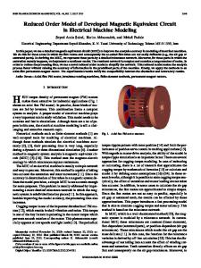
The second modeling approach available in the literature is a moving boundary approach (MB). This approach, originally proposed by [8], divides the heat exchanger into time-varying control volumes, corresponding to the phase of the fluid. For example, a typical condenser would be divided into three regions: superheated vapor, two-phase fluid, and subcooled liquid. For each region the conservation equations are applied, and parameter values are lumped for each fluid region. The resulting model is of relatively low order, captures the salient dynamic behavior, but requires the modeler to define many effective parameters. While some of these lumped parameters have known bounds, the possible range of values can vary significantly. For example, the heat transfer coefficient for the two-phase fluid can vary by more than an order of magnitude (Fig. 6). Although the MB approach results in a minimal representation of the system dynamics [7], accurate prediction relies on extensive tuning of the effective model parameters. Nonlinear Finite Control Volume Model
Linearization of FCV Models
Decompose by Dynamic Mode Type
II. MOVING BOUNDARY HEAT EXCHANGER MODELS The moving boundary (MB) approach to multi-phase heat exchanger modeling relies on several fundamental assumptions. First, despite the complexity of typical heat exchanger geometries (Fig. 4), the MB approach assumes one-dimensional fluid flow through a horizontal tube, with equivalent mass, surface areas, length, and volume (Fig. 5). Axial conduction is neglected, as is the pressure drop due to change in momentum (i.e. pressure is assumed to be uniform throughout the heat exchanger).
Numerical Model Reduction Validation of Moving Boundary Models Extract Physical Parameters of Reduced Order Model
Nonlinear Moving Boundary Model
Integrate Lumped Parameter Maps into MB Models
extracted from the reduced order equations, using knowledge of the final equation form to recover the physical significance of the numerically reduced order model. This approach is repeated for a range of operating conditions, and a nonlinear parameter map is created, and incorporated into the nonlinear MB model. The remainder of this paper is organized as follows. Moving Boundary and Finite Control Volume evaporator models are presented in Sections 2 and 3. The derivation of the FCV model as a set of Ordinary Differential Equations (ODEs), rather than the typical set of Differential-Algebraic-Equations (DAEs) is a notable contribution in itself, and differs from most existing FCV models in the literature. Linearization of both models is performed, but space constraints prevent the lengthy presentation of the resulting equations. Section 4 presents the lumped parameter identification procedure, and illustrates how the nonlinear parameter maps are constructed. The paper concludes with some remarks regarding the novelty and potential impact of the approach.
Generate Parameter Maps For Entire Operating Range
Figure 3: Parameter Identification Process
This paper seeks to bridge the gap between these two modeling paradigms by utilizing the more complex FCV models to determine the optimal choice of effective MB model parameters to ensure dynamic similarity between the more accurate FCV models, and the more control-oriented MB models. This process is illustrated in Fig. 3. Utilizing detailed information about the heat exchanger geometry and empirical correlations for distributed parameters, nonlinear FCV models are constructed using 1st principles. These are then linearized about a selected operating condition, and decomposed according to the dynamic mode type (e.g. conservation of refrigerant energy). Numerical model reduction techniques are used to then reduce the number of dynamic modes to describe each mode type for each region. The effective physical parameters are then
Figure 4: Actual heat exchanger with multiple distribution paths and varied geometry Quality = 1 Twall,1(t)
Twall,2(t)
m& inhin
P(t)
Qualityin > 0 Two-Phase
Single-Phase
L1(t)
L2(t) LTotal
Figure 5: Idealized heat exchanger geometry
1450
& outhout (t) m
∂t
∂z & ∂ ( ρAh − AP ) ∂ (mh ) + = piα i (Tw − Tr ) ∂t ∂z (C p ρA)w ∂Tw = piα i (Tr − Tw ) + poα o (Ta − Tw ) ∂t
(2) (3)
d z 2 (t ) ∂f (z, t ) dz = ⎡ ∫ f ( z, t )dz ⎤ ⎥⎦ (4) dt ⎢⎣ z1 (t ) ∂t d (z2 (t )) d ( z1 (t )) − f (z2 (t ), t ) + f ( z1 (t ), t ) dt dt Due to space constraints, only selected results are presented here. The interested reader is referred to [14] for a complete derivation of each of the equations and the associated nomenclature. For example, the conservation of refrigerant energy as applied to the two-phase regions is given in Eq. 5. z 2 (t )
∫ () z1 t
execute in real-time. However, the necessary information to construct a detailed dynamic FCV model can be assumed to be available. In this paper, we focus on the following: Heat Exchanger Geometry – Modern heat exchangers employ a variety of techniques to maximize heat transfer. In particular, the heat exchanger may use multiple fluid paths, which may branch into additional paths as the fluid evaporates to accommodate the increasing volume of fluid. Thus this changing geometry will affect several key physical parameters such as surface areas and crosssectional areas, and cannot be included in the MB models. Fluid Property Profiles – The MB method assumes average temperatures of the refrigerant and heat exchanger metal, effective two-phase fluid properties, such as enthalpy and density, and average single-phase properties. In reality, temperatures vary continuously throughout the heat exchanger, and slight variations in assumed two-phase properties can have a dramatic impact. For example, a 1% change in mean void fraction (an effective parameter used to characterize the two phase fluid), can result in more than a 30% change in the total refrigerant mass assumed in the heat exchanger, which can greatly influence the dominant time constants of the system. 5
Heat Transfer Coefficient
The standard derivation procedure requires the integration of the governing PDEs given in Eqs. 1-3 along the length of the heat exchanger to remove spatial dependence. The integration rule given in Eq. 4, commonly known as Leibniz’s equation, is used to handle the timevarying boundary between the fluid regions. This approach can be tedious and requires a significant amount of algebraic manipulation. With some minor differences many authors use some form of this approach to model an evaporator in a subcritical cycle [9],[10],[11],[4],[12],[13]. The fluid is assumed to enter as a two-phase mixture, and leave as a superheated vapor, and thus the model is divided into two regions. This model assumes a time-invariant mean void fraction in the two-phase region [9]. ∂ρA ∂m& (1) + =0
d (ρ h ) ⎞ ⎛ d (ρ f h f ) ⎜⎜ (1 − γ ) + g g (γ ) − 1⎟⎟ Acs L1P&e + (ρ g hg − ρ f h f )Acs L1γ& ( 5 ) dP dP e e ⎠ ⎝ ⎛ L ⎞ + (ρ f h f − ρ g hg )(1 − γ )Acs L&1 + m& int hint − m& in hin = α i Ai ⎜⎜ 1 ⎟⎟(Tw1 − Tr1 ) ⎝ LTotal ⎠
The final model can be written in the nonlinear state space form in Eq. 6 with the states and input vectors defined in Eqs. 7 and 8 respectively. A complete derivation and linearization, can be found in [15]. (6) Z ( x, u ) ⋅ x& = f ( x, u ) x = [L1 u = [m& in
Pe m& out
hout
Tw1 Tw2 ]
hin Tair ,in
T
T m& air ]
(7) (8)
III. FINITE CONTROL VOLUME HEAT EXCHANGER MODELS While several of the assumptions for the MB model are also applied to the FCV models, there is the potential for much greater accuracy due to more realistic geometric and parametric representations. Many in the HVAC industry have developed extremely detailed and accurate, if proprietary, steady state models of heat exchangers. Understandably, the dynamic counterparts to these models have found less use given their complexity and inability to
Variation of Heat Transfer Coefficient with Quality
4 Dobson-Chato Correlation
3 2 1 0 0
Wattelet-Chato Correlation
0.2
0.4
Quality
0.6
0.8
1
Figure 6: Plot of Heat Transfer Coefficient for Evaporating/Condensing Flows
Heat Transfer Coefficients – Extensive and ongoing research attempts to develop empirical correlations for the rate of heat transfer as a function of temperature, pressure, fluid phase, heat flux, passage geometry, etc. For example, the Wattelet-Chato correlation for evaporating flows [16], and the Dobson-Chato correlation for condensing flows [17] are shown in Fig. 6. Note that the heat transfer coefficient can change by an order of magnitude as the fluid changes phases (fluid quality is a relative measure of vapor and liquid content in a two-phase flow). FCV models have been presented previously in the literature (e.g. [2],[18],[19]). However, because of the multi-time scale dynamics present, the governing equations are generally represented as a system of DifferentialAlgebraic-Equations (DAEs). In this paper, we present a
1451
derivation wherein the governing equations are represented as a set of Ordinary Differential Equations (ODEs). The same governing PDEs described in Eqs. 1-3 are utilized, and integrated to remove spatial dependence. Although the resulting equations use lumped parameters for each assumed control region, by increasing the number of control volumes (i.e. increasing the level of discretization), the model approximates the distributed parametric nature of a real heat exchanger (Fig. 7). Assuming that the heat exchanger has been discretized into ‘n’ regions, the equations for conservation of refrigerant energy, conservation of heat exchanger wall energy, and conservation of refrigerant mass are shown in Eqs. 9-11. Tw , k
Tw,1 m& in
hin
m& e,1 he,1 h1
⎡ ⎛ ∂ρ Z 22 = ⎢V1 ⎜ 1 ⎢⎣ ⎜⎝ ∂h1
{[
Figure 7: FCV Evaporator Model Diagram
⎡U& 1 ⎤ ⎡ m& in hin − m& 1 h1 + α i ,1 Ai ,1 (Tw,1 − Tr ,1 ) ⎤ ⎢ ⎥ ⎢ ⎥ M ⎢ M ⎥=⎢ ⎥ ⎢U& n ⎥ ⎢m& n −1 hn −1 − m& out hout + α i , n Ai , n (Tw, n − Tr ,n )⎥ ⎣ ⎦ ⎣ ⎦
(9)
0 O ⎛ ∂ρ n −1 ⎜ (hn −1 − hn )⎜ ⎝ ∂hn −1
⎛ ⎞ ⎟ L Vn ⎜ ∂ρ n ⎟ ⎜ ∂hn P⎠ ⎝
⎞ ⎟V n −1 ⎟ P ⎠
⎞⎤ ⎟⎥ ⎟ P ⎠⎥ ⎦
(C m) ]} A (T − T ) p
w, n
[
m& out
hin
Ta ,in
m& air
]
T
( 13 )
the left hand side of Eqs. 9 and 10 can be expanded resulting in a nonlinear state space form in Eq. 6. The elements of Z (x, u ) and f (x, u ) matrices are given as: ⎡ Z 11 Z ( x, u ) = ⎢⎢ Z 21 ⎢⎣ 0
Z 12 Z 22 0
0 ⎤ ; 0 ⎥⎥ Z 33 ⎥⎦
⎡ ⎛ ∂ρ Z 21 = ⎢V1 ⎜ 1 ⎜ ⎣⎢ ⎝ ∂P
( 19 )
Oil Return Line
( 11 )
Similar to the MB models, the conservation of mass equations are substituted into the conservation of refrigerant energy equations to eliminate intermediate mass flow variables, resulting in a single conservation of mass equation for the entire heat exchanger. A transformation of state variables is applied to facilitate the linearization. Selecting the states and inputs as: T ( 12 ) x = [Pe he,1 K he, n Tw,1 K Tw, n ] u = m& in
( 18 )
Space constraints preclude a description of the linearized model; however, the straightforward, albeit tedious, process is similar to that found in [14].
⎡ E& w,1 ⎤ ⎡ α o ,1 Ao ,1 (Ta ,1 − Tw,1 ) − α i ,1 Ai ,1 (Tw,1 − Tr ,1 ) ⎤ ⎢ ⎥ ⎢ ⎥ ( 10 ) M ⎢ M ⎥=⎢ ⎥ ⎢ E& w, n ⎥ ⎢α o , n Ao , n (Ta , n − Tw, n ) − α i , n Ai , n (Tw, n − Tr , n )⎥ ⎦ ⎣ ⎦ ⎣
⎡ m& e ,1 ⎤ ⎡ m& in − m& 1 ⎤ ⎢ ⎥ ⎢ ⎥ M ⎢ M ⎥=⎢ ⎥ ⎢⎣m& e,n ⎥⎦ ⎢⎣m& n−1 − m& out ⎥⎦
0 ⎤ ⎥ 0 ⎥ ( 17 ) ⎥ 0 ⎥ ⎥ Vn ρ n ⎥ ⎥ ⎦
m& in (hin − h1 ) + α i ,1 i ,1 w,1 r ,1 ⎤ ⎡ ⎥ ⎢ M ⎥ ⎢ ⎢ m& in (hn −1 − hout ) + α i ,n Ai ,n (Tw,n − Tr ,n ) ⎥ ( 20 ) ⎥ ⎢ m& in − m& out f ( x, u ) = ⎢ ⎥ ⎢ α o ,1 Ao ,1 (Ta ,1 − Tw,1 ) − α i ,1 Ai ,1 (Tw,1 − Tr ,1 ) ⎥ ⎥ ⎢ M ⎥ ⎢ ⎢α A (T − T ) − α A (T − T )⎥ i , n i , n w, n r ,n ⎦ ⎣ o , n o , n a , n w,n
m& e,n m& out he,n hout
hn −1
0
Z 33 = diag (C p m )w,1 L
Tw , n
m& e,k he,k hk
hk −1
Z 12
V1 ρ 1 0 ⎡ ⎢ ⎛ ∂ρ 1 ⎞ ⎟V ⎢ (hin − h1 )⎜ O ⎜ ∂h ⎟ 1 ⎢ ⎝ 1 P⎠ =⎢ M O ⎢ ⎢(h − h )⎛⎜ ∂ρ 1 ⎞⎟V L n ⎜ ⎢ n −1 ⎟ 1 ⎝ ∂h1 P ⎠ ⎣
⎡ − V1 ⎤ Z 11 = ⎢⎢ M ⎥⎥ ⎢⎣− Vn ⎥⎦
⎛ ⎞ ⎟ + L + Vn ⎜ ∂ρ n ⎟ ⎜ ∂P h1 ⎠ ⎝
⎞⎤ ⎟⎥ ⎟⎥ hn ⎠ ⎦
(14 & 15 )
( 16 )
Figure 8: Experimental Vapor Compression System
To validate the models, a simple subcritical vapor compression system is used (Fig. 8). This test apparatus has variable control of the electronic expansion valves (EEVs), compressor, and flow valves for the secondary fluid (water). The system uses R134a, and is fully equipped with pressure, temperature, and flow transducers. Experimental results for step changes in compressor speed are shown compared with the model predictions (Fig. 9), illustrating that the efficacy of the model. The FCV model was examined for dependency on the selected number of regions. As expected, the predicted transients increased in accuracy for increasing levels of discretization, with the simulation results virtually indistinguishable at higher discretization levels. Fig. 10 shows the pressure response in a straight tube evaporator for a step change in expansion valve opening, for FCV models with 2, 8, 12, and 15 control volumes. While few regions are required for this deliberately simple geometry, higher levels of discretization would be appropriate for more realistic heat exchanger configurations.
1452
This system is decomposed in order to isolate the individual dynamic modes. For example, for the conservation of wall energy modes, we write: ⎡ U ⎤ ⎥ ⎢ ( 24 ) & Ew = [ AEE ]Ew + [ AEU AEm BE ]⎢mtotal ⎥; yE = [I ]Ew ⎢ u ⎥ ⎦ ⎣
240 Data FCV Evaporator
Pressure
235
230
225
Thus the vector of refrigerant energies (i.e. profile of refrigerant temperatures) and total refrigerant mass are considered inputs to the wall energy subsystem, and the outputs of interest are the vector of wall energies (i.e. profile of heat exchanger wall temperatures). Standard model reduction techniques [20] are now applied to this subsystem. For example, reducing the above system to a single state, the reduced order system ⎡ U ⎤ ⎢ ⎥ ( 25 ) x& rE = [ ArE ]xrE + [BrE1 BrE 2 BrE 3 ]⎢mtotal ⎥ ⎢⎣ u ⎥⎦
220
215 0
50
100
150
200 250 Time
300
350
400
450
Figure 9: Experimental validation of FCV simulations for step changes in compressor speed. 305 FCV - 2 regions FCV - 8 regions FCV - 12 regions FCV - 15 regions
Pressure (kPa)
304 303
y rE = [C rE ]xrE
would correspond to a lumped parameter 1st order system whose dynamic behavior is closest to the discretized system. Repeating this procedure for the refrigerant energy states, and reassembling, results in the 3rd order system: BrU 2 BrU 1CrE ⎤ ⎡ xrU ⎤ ⎡ BrU 3 ⎤ ⎡ x& rU ⎤ ⎡ ArU ⎢m& ⎥ = ⎢ 0 0 0 ⎥⎥ ⎢⎢mtotal ⎥⎥ + ⎢⎢ Bm ⎥⎥u ⎢ total ⎥ ⎢ ( 26 ) ⎢⎣ x& rE ⎥⎦ ⎢⎣ BrE1C rU BrE 2 ArE ⎥⎦ ⎢⎣ xrE ⎥⎦ ⎢⎣ BrE 3 ⎥⎦
302 301 300 299 0
20
40
60 Time (sec)
80
100
⎡ xrU ⎤ C E C rE ]⎢⎢mtotal ⎥⎥ + [D ]u ⎢⎣ xrE ⎥⎦
Figure 10: FCV simulations for different discretization. Response of evaporator pressure for step changes in valve opening
y = [CU C rU
IV. LUMPED PARAMETER TUNING VIA NUMERICAL MODEL REDUCTION
Noting that the total energy across all regions is given by:
The FCV model presented in the previous section can be linearized with the state variables Eq. 12, and denoted: x& = Ax + Bu ( 21 ) y = Cx + Bu Using the matrix Z(x,u) defined in Eq. 14-19 as a state transformation matrix, a linearized system representation is obtained with states corresponding to the refrigerant energy, refrigerant mass, and heat exchanger wall energy: T ( 22 ) x = [U 1 K U n mtotal E w,1 K E w,n ] Noting that the conservation of mass equation is a pure integration, and resulting state space representation is: ⎡ U& ⎤ ⎡ AUU ⎢ ⎥ ⎢ ⎢m& total ⎥ = ⎢ 0 ⎢ E& ⎥ ⎢ A ⎣ w ⎦ ⎣ EU y = [CU
Cm
AUm 0 AEm
AUE ⎤ ⎡ U ⎤ ⎡ BU ⎤ ⎢ ⎥ 0 ⎥⎥ ⎢mtotal ⎥ + ⎢⎢ Bm ⎥⎥u AEE ⎥⎦ ⎢⎣ E w ⎥⎦ ⎢⎣ BE ⎥⎦
⎡ U ⎤ ⎢ ⎥ C E ]⎢mtotal ⎥ + [D ]u ⎢⎣ E w ⎥⎦
( 23 )
Cm
[ ] [ ] = [1 ]E = [1 ]C
U total = 11×n U = 11×n CU xrU E w,total
1×n
1×n
w
( 27 )
E xrE
we define a state transformation matrix of:
{[[ ]
T = diag 11× n CU
[ ] ]}
1 11× n CE
( 28 )
which will recover the physical significance of the state variables. This final 3rd order model is compared to the known lumped parameter linearization, in order to identify critical parameters. For example, the reduced order numerical value given by ArE can be equated to lumped parameters as: ⎛ α A + α o Ao ⎞ , ( 29 ) ⎟ ArE = −⎜ i i ⎜ ⎟ C m p ⎝ ⎠ and similarly: ⎞ ⎛ ( 30 ) ([11×n ]CU )(BrU 1CrE )([11×n ]C E )−1 = ⎜⎜ αCi Ami ⎟⎟ ⎝ p ⎠ Continuing this process, utilizing the subset of parameters with known values, values for the unknown parameters, such as including internal and external heat transfer coefficients, can be obtained. By incorporating
1453
these parameter estimates into the MB models, the time and data intensive step of parameter tuning can be eliminated. Moreover, this process of FCV model generation, linearization, reduction, and parameter extraction can be automated. Thus by repeating the parameter identification process for the range of operating conditions, numerical parameter maps can be generated. These are then integrated into the moving boundary models to ensure the accuracy of the models across the entire operating envelope. Figure 11 demonstrates the efficacy of this approach. Simulation results for evaporator pressure and superheat are shown for the high order FCV models, and for the low order MB models for both estimated and identified values of heat transfer coefficient. The MB models using the identified parameters show considerable improvement in the accuracy, while retaining the computational and mathematical simplicity of the low order model. 307
MB Untuned MB Tuned FCV - 15 regions
306
REFERENCES [1] [2] [3]
[4]
[5] [6] [7]
[8]
Pressure (kPa)
305 304
[9]
303 302
[10] 301 300 299 0
[11] 20
40
60 Time (sec)
80
100
Figure 11: FCV vs. MB simulations for tuned/untuned parameters
V. CONCLUSIONS
[12]
[13]
This paper makes several key contributions to the study of vapor compression system dynamics. The existing lumped parameter moving boundary approach has been presented, which provides a simple method to obtain low order models. A finite control volume approach is presented, avoiding the standard system of DAEs, and creating a set of nonlinear ODEs. This framework allows inclusion of parametric details omitted by the simpler models. This model is validated against experimental data. Finally, an approach for extracting the most effective choice of lumped parameters for the moving boundary models has been introduced, and can be used to generate nonlinear parameter maps over a larger operating range. The resulting low order model is dynamically similar to higher order models with distributed parameter values. ACKNOWLEDGEMENTS
[14] [15] [16] [17] [18] [19] [20]
The authors are pleased to acknowledge the support of NSF CAREER award CMMI-0644363.
1454
Anonymous, "Annual Energy Review 2005," DOE/EIA0384(2005), Jul 2006. W.D. Gruhle and R. Isermann, "Modeling and Control of a Refrigerant Evaporator," ASME J. of Dynamic Systems Measurement & Control, vol. 107, no. 4, pp. 235-240, Dec, 1985. E.W. Grald and J.W. MacArthur, "A Moving-Boundary Formulation for Modeling Time-Dependent Two-Phase Flows," Int. J. of Heat & Fluid Flow, vol. 13, no. 3, pp. 266-272, Sep, 1992. X.D. He, S. Liu, and H. Asada, "Modeling of Vapor Compression Cycles for Multivariable Feedback Control of HVAC Systems," ASME J. of Dynamic Systems Measurement & Control, vol. 119, no. 2, pp. 183-191, Jun, 1997. B.P. Rasmussen and A. Alleyne, "Control-Oriented Modeling of Transcritical Vapor Compression Systems," ASME J.of Dynamic Systems, Meas., and Ctrl, vol. 126, no. 1, pp. 54-64, Mar, 2004. Bendapudi, S. and Braun, J.E., "A Review of Literature on Dynamic Models of Vapor Compression Equipment," ASHRAE Report #4036-5, May 2002. B.P. Rasmussen, A.G. Alleyne, and A.B. Musser, "Model-Driven System Identification of Transcritical Vapor Compression Systems," IEEE Trans. on Control Systems Technology, vol. 13, no. 3, pp. 444-451, 2005. G.L. Wedekind, B.L. Bhatt, and B.T. Beck, "A System Mean Void Fraction Model for Predicting Various Transient Phenomena Associated With Two-Phase Evaporating and Condensing Flows," Int. J. of Multiphase Flow, vol. 4, no. 1, pp. 97-114, Mar, 1978. B.T. Beck and G.L. Wedekind, "A Generalization of the System Mean Void Fraction Model for Transient Two-Phase Evaporating Flows," ASME J. of Heat Transfer, vol. 103, no. 1, pp. 81-85, Feb, 1981. J. Chi and D. Didion, "A Simulation Model of the Transient Performance of a Heat Pump," Int. J. of Refrigeration, vol. 5, no. 3, pp. 176-184, May, 1982. P.M.T. Broersen and M.F.G. van der Jagt, "Hunting of Evaporators Controlled by a Thermostatic Expansion Valve," ASME J. of Dynamic Systems, Meas., and Ctrl, vol. 102, no. 2, pp. 130-135, Jun, 1980. M. Willatzen, N.B.O.L. Pettit, and L. Ploug-Sorensen, "General Dynamic Simulation Model for Evaporators and Condensers in Refrigeration, Part I," Int. J. of Refrigeration, vol. 21, no. 5, pp. 398-403, Aug, 1998. J.M. Jensen and H. Tummescheit, "Moving Boundary Models for Dynamic Simulations of Two-Phase Flows," in Proceedings of the 2nd International Modelica Conference, 2002, pp. 235-244. B.P. Rasmussen, "Dynamic Modeling and Advanced Control of Air Conditioning and Refrigeration Systems," Dept. of Mech. and Ind. Eng., University of Illinois, Urbana, IL, Dec. 2005. B.P. Rasmussen, "Dynamic Modeling and Advanced Control of Air Conditioning and Refrigeration Systems," Dept. of Mech. Eng., University of Illinois, Urbana, IL, Sept. 2005. Wattelet, J.P., "Heat transfer flow regimes of refrigerants in a horizontal - tube evaporator," University of Illinois at UrbanaChampaign, ACRC TR-55, 1994. M.K. Dobson and J.C. Chato, "Condensation in Smooth Horizontal Tubes," J. of Heat Transfer, vol. 120, no. 2, pp. 193213, 1998. J.W. MacArthur, "Transient Heat Pump Behaviour: a Theoretical Investigation," Int. J. of Refrigeration, vol. 7, no. 2, pp. 123-132, Mar, 1984. Bendapudi, S. and Braun, J.E., "Development and Validation of a Mechanistic, Dynamic Model for a Vapor Compression Centrifugal Chiller," ASHRAE Report #4036-4, May 2002. Skogestad, S. and Postlethwaite, I. Multivariable Feedback Control: Analysis and Design, NY: John Wiley & Sons, 1996.