compact representation for the visual data using a set of parameterized basis (wavelet) functions, ... components analysis (PCA) [1,2] adopts a low-dimensional.
Parametric Representations for Nonlinear Modeling of Visual Data Ying Zhu†
Dorin Comaniciu‡
Visvanathan Ramesh‡
†Electrical
Engineering Princeton University Princeton, NJ 08544
Abstract Accurate characterization of data distribution is of significant importance for vision problems. In many situations, multivariate visual data often spread into a nonlinear manifold in the high-dimensional space, which makes traditional linear modeling techniques ineffective. This paper proposes a generic nonlinear modeling scheme based on parametric data representations. We build a compact representation for the visual data using a set of parameterized basis (wavelet) functions, where the parameters are randomized to characterize the nonlinear structure of the data distribution. Meanwhile, a new progressive density approximation scheme is proposed to obtain an accurate estimate of the probability density, which imposes discrimination power on the model. Both synthetic and real image data are used to demonstrate the strength of our modeling scheme.
1. Introduction We address the problem of learning parametric models from multivariate data. In many pattern recognition and vision applications, an interesting pattern is measured or visualized through multivariate data such as time signals and images. Its random occurrences are described as scattered data points in the high-dimensional space. For accurate representation and effective use of the decisive information, it is important to explore the intrinsic low dimensionality of the scattered data and to obtain an accurate statistical model for the data distribution. The general procedure of parametric modeling approximates the data distribution with a family of parameterized density models and then estimates model parameters for the best fit to the data. Among the commonly used techniques, principal components analysis (PCA) [1,2] adopts a low-dimensional linear representation and approximates the multivariate data by a low rank Gaussian density model. Linear factor analysis [3] approximates class distribution as a Gaussian distribution with structured covariance matrix. These linear modeling schemes are capable of representing the data distributions with ellipsoidal shape, but they are unable to handle the situations where data samples spread into a nonlinear manifold that is no longer Gaussian. The nonlinear structure of multivariate data distribution is not unusual even when the internal decisive variables of the pattern have a unimodal distribution. For example, images of an object under varying poses form a nonlinear manifold in the high-dimensional
Stuart Schwartz†
‡Imaging
& Visualization Department Siemens Corporate Research 755 College Road East, Princeton, NJ 08540 space. The expression variation can lead to structural nonlinearity on the data distribution of single view face images. Similar situation happens when we model the images of cars with a variety of outside designs. One way to handle the nonlinearity is through multimodal approximation using a mixture density model [4, 5]. Alternative methods have been proposed to directly identify the nonlinear principal manifold [6, 7, 22, 23]. However, no probabilistic model is associated with these approaches. This paper presents a new statistical modeling scheme that not only characterizes the nonlinear structure of the data distribution but also represents it with a probabilistic distribution model. The modeling scheme is built by defining a parametric function representation for multivariate data. We statistically model the random function parameters to obtain a density estimate of the data distribution. Compared to other nonlinear modeling schemes, the probabilistic distribution model obtained by our scheme provides a likelihood measure therefore has the discrimination power essential for pattern identification. The paper is organized as follows. In section 2, we introduce the parametric function representation for multivariate data. In section 3 and 4, a new progressive density approximation scheme is proposed to obtain the probabilistic distribution function. Experimental results on both synthetic and real data are presented in section 5. We finish with conclusions and discussions in sections 6.
2. Parametric function representation In addition to the traditional vector representation y ∈ R n for n-dimensional multivariate data, we associate a smooth function for every data sample. A length-n vector y = [ y1 , L y n ]T is associated with a smooth function
y(t ) ∈ L2 : R1 → R1 (t ∈ R1 ) interpolated from its discrete components y (t i ) = y i (i = 1, L , n) . When the multivariate data are images, functions defined on R2 , y (t ) ∈ L2 : R 2 → R 1 (t = (t1 , t 2 ) ∈ R 2 ) , are adopted for the representation. The function association applies a smoothing process to the discrete data components and is unique when only smooth functions are involved. In practice, these functions may be immediately available from data generating process. As a result, in the function space L2 , there is a counterpart of the scattered multivariate data located in vector space.
Compared with linear representation in PCA or Gaussian mixtures model, the advantage of function association lies in its ease to handle the non-linearity by parametric effects embedded in the data. It has intensive use in functional data analysis [8,9,19] for recovering principal curves in 1D signals. In [6], spline functions are used to parameterize the nonlinear principal manifold of an arbitrary data distribution. In [10], the parametric representation also provides a highlevel semantic description of the pattern. n
Visual data space
2
R
L
y
y(t)
Function space
the domain of x to the domain of parameter set denoted by R p , g p : Rm → R p , g p (x) = [W N (x), Θ N (x)]T
(3)
By defining the matrix b (t 1 ; θ i ) (4) M B(Θ N ) = [b (θ 1 ), L , b(θ N )] where b(θ i ) = b(t n ; θ i ) the multivariate data y is related to x as T
p
= [b(θ 1 (x)), L , b(θ N (x))]⋅ W N (x) + n
R gp
x
L2 , g f : R m → L2 , or equivalently, as a mapping g p from
y = [ y1 , L , y n ]
gf m
R Data-generating space
a mapping g f from the domain of x to the function space
{W,Θ}
Parameter space
Figure 1. Parametric function representation through space mappings. Multivariate data y is represented in function form y(t) parameterized by {W,Θ}.
Figure 1 illustrates the idea of parametric function representation. Let {bθ } be a base set for the function space L2 . The basis function bθ (t ) = b(t; θ ) : R d → R (t ∈ R d ) is parameterized and indexed by parameter θ , where θ can take a continuous range of values. Examples of such base sets include wavelets, splines and trigonometric functions. Any function y (t ) ∈ L2 can be closely approximated by a sufficient number (N ) of basis functions,
b (t ; θ 1 ) y (t ) ≅ [ w1 , L w N ] ⋅ M b(t; θ N )
(1)
The basis function b(t; θ ) is generally nonlinear in θ . Once the basis b is chosen, the function y (t ) is completely determined by the linear parameter set {w1 , L , wN } and the nonlinear set {θ 1 , L ,θ N } . The vector notations W N , Θ N , and Θ N for the linear, nonlinear and overall parameter sets, are used in the following discussions, where N denotes the number of basis functions involved. w1 θ1 Θ N −1 (2) W N = M ; Θ N = M ; Θ N = w N w N θ N θ N To study data distribution, we assume x ∈ R m , in a vector form, to be the underlying quantities with minimum dimension (intrinsic dimensionality) that govern the datagenerating process. Each observed data point reflects an occurrence of x . Our goal is to statistically characterize x using the observed data y . With parametric function association, the data-generating process can be formulated as
(5)
= B(Θ N (x)) ⋅ W N (x) + n where n is introduced to account for the noise in the observed data as well as the representation error. By choosing a proper type of basis functions, (5) defines a compact representation for multivariate data, and modeling the data distribution can be resolved through modeling the parameter set Θ N .
3. Statistical modeling through progressive distribution approximation Based on the parametric function representation (5), here we discuss algorithms and criteria for modeling the data distribution. In most situations with a single pattern involved, the governing factor x is likely unimodal although the observed data y may disperse into a nonlinear manifold due to parametric effects. Our discussion is primarily restricted to such internally unimodal data clusters. Figure 2 shows a toy example. The observed multivariate data y = [ y1 , L , y n ]T consists of n equally spaced samples from a random process y (t ; w,θ ) , y i = y (t i ; w, θ ); (t i = i ⋅ T ) y (t ; w, θ ) = w ⋅ b(t ; θ ); (θ = ( s, t 0 )) t − t0 ) (6) s where w , s and t 0 are random variables with normal distributions. The data-generating process is characterized by these three intrinsic parameters. Figure 2(a) plots a few data samples in the form of time signals. Figure 2(b) shows the nonlinear structure of the data distribution by plotting the data projections on their first two linear principal components. The linear PCA and multimodal approximation are either incapable of or inefficient in modeling such distribution, even though the distribution of the internal variables {w, s, t 0 } is simply Gaussian. Such phenomenon is familiar to many situations where the visual data is generated by a common pattern and bears similar features up to small b(t ; θ ) = (t − t 0 )exp(−
yi
P2
Density Estimate
Introduce new basis function
EM/MLE
No P1 t (b) (a) Figure 2. Nonlinearly distributed manifold. (a) Curve samples. (b) 2D visualization of the data distribution.
random deformation. The framework of our modeling scheme is shown in Figure 3. The basic idea is to characterize the nonlinear structure of internally unimodal distributions by modeling the parametric effects. Equation (6) defines a single wavelet function denoted as the Derivative of Gaussian (DOG) function. In practice, visual data is more complicated and requires more basis functions to encode (1). These basis functions are parameterized with randomized parameters to accommodate random deformation. Wavelet functions are primarily used in this work for compact encoding of visual data. As the basis functions are gradually introduced, a sequence of density estimates, which approach the true data distribution, is also obtained.
3.1. Statistical modeling From (3), both W N and Θ N are determined by x through the mapping g p . Assuming that x is well modeled by normal distribution and the mapping g p is smooth, the linearization of W N (x) and Θ N (x) is valid around the mean of x . W N (x) = W N , 0 + AW , N ⋅ x (7) Θ N (x) = Θ N , 0 + AΘ, N ⋅ x In practice, if prior knowledge shows that the assumption of normality or linearization does not hold well, we can always replace the normal distribution with a more suitable unimodal distribution form for x and include higher order terms in (7). The following discussion remains the same. However, to simplify the analysis, we keep normal distribution as nominal distribution for x and assume that linearization (7) is valid. Consequently, multivariate data y is effectively modeled by a jointly Gaussian distribution of W N and Θ N through (5).
p(y ) = ∫ p (W N , Θ N ) ⋅ p(y | W N , Θ N )dW N dΘ N
(8)
WN Θ N
Based on this conclusion, the following discussion is devoted to finding the particular distribution from the family defined by (8) that best fits the observed data set. Assume that n (5) is white Gaussian noise with zero mean and variance σ 2N and {W N (x), Θ N (x)} has joint mean µ N
Stopping rule?
Yes
Stop
Figure 3. Proposed modeling framework. Basis functions are gradually added into the data representation until the stopping criterion is satisfied.
and covariance matrix Σ N , n ~ N (0, σ N2 ⋅ I n )
(9)
W N Θ ~ N ( µ N , Σ N ) N
(10)
Denote Φ N = {µ N , Σ N , σ N2 } . Equations (8)-(10) define a family of density functions parameterized by Φ N . Given M independently identical distributed data samples {y 1 , L , y M } , the density estimate pˆ (y ) , in the maximum likelihood (ML) sense, is then defined by the ML estimate of Φ N such that the likelihood
p(y 1 , L , y M | Φ N ) = ∏ii ==1M p(y i | Φ N ) is maximized over the parameterized family (8), ˆ ) pˆ (y ) = p(y | Φ N ˆ = argmax ∏ M p (y | Φ) Φ N
where ΩN
Φ∈Ω N
i =1
(11)
(12)
i
denotes the domain of Φ N . Within the
framework of ML estimation, Φ N = {µ N , Σ N , σ N2 } defines the hyper-parameter set. To solve (12), we need to answer two questions. First, how many basis functions should be used. We address this issue by introducing a progressive density approximation scheme. Second, given N , how to find basis functions with randomized parameters and solve the ML estimation (12). We answer this question in section 4.
3.2. Progressive density approximation Involving more basis functions may increase the effective dimension of the model (8)-(10), i.e. the dimensionality of Θ N , as well as the computational load. On the other hand, the involvement of more basis functions extends the parametric family of distributions (8) and therefore may increase the accuracy of density estimation (12). Intuitively, N should be large enough to assure the accuracy of density estimation. Meanwhile, N should be bounded to avoid overfitting.
Before introducing the progressive density approximation method, we first derive a measurement for the accuracy of density estimation. Assume p t (y ) is the true density
Pt
pˆ N −1
function for the observed data samples {y 1 , L , y M } , and pˆ (y ) is the estimated density. The Kullback-Leibler divergence D ( p t || pˆ ) is an effective measure to evaluate the similarity between the two density functions, p (y ) dy D ( p t || pˆ ) = ∫ p t (y ) ⋅ log t pˆ (y ) = E pt [log p t (y )] − E pt [log pˆ (y )]
(13)
D ( p t || pˆ ) is nonnegative and equal to zero only when the two densities coincide. Since the term E pt [log p t (y )] is independent of the density estimate pˆ (y ) , an equivalent similarity measurement can be defined as L( pˆ ) = E pt [log pˆ (y )] = − D( p t || pˆ ) + E pt [log p t (y )]
(14)
≤ E p t [log p t (y )]
pˆ 0
pˆ N
…
ΩN-1
ΩN
pˆ N +1
…
ΩN+1
Figure 4. Progressive density approximation. A sequence of density estimate pˆ N progressively approaches the true density function pt as more basis functions are introduced.
L ≤ Lˆ ( pˆ N −1 ) ≤ Lˆ ( pˆ N ) ≤ Lˆ ( pˆ N +1 ) ≤ L
(18) This indicates that the sequence of density estimates { pˆ N } progressively approaches the true density. To avoid overfitting, a practical stopping rule is to examine the increasing of Lˆ ( pˆ N ) and stop at the point where the increasing of Lˆ ( pˆ ) saturates. N
4. Hyper-parameter estimation
L( pˆ ) increases as estimated density pˆ gets closer to the true density pt . It is upper bounded by E pt [log p t (y )] . Since pt is unknown, L( pˆ ) , the expectation of log pˆ (y ) , can be estimated in practice by its sample mean. 1 M Lˆ ( pˆ ) = (15) ∑i =1 log pˆ (y i ) M Figure 4 illustrates the process of density estimate. By introducing more basis functions, the density estimate gradually approaches the true distribution. The algorithm is summarized below. A similar idea of progressive density approximation is also found in a recent work [11] where the basic components directly modify the density function. Progressive Density Approximation Step 1: Start with N = 1 . Step 2: Find the ML density estimate pˆ N (12). Step 3: Increase N by 1, and repeat Step 2 until the stopping rule is satisfied. Fact: pˆ N gets closer to the true density pt as N increases. The algorithm produces a sequence of density estimates { pˆ 0 , pˆ 1 , L , pˆ N , L} , ˆ ) pˆ N (y ) = p(y | Φ and N (16) ˆ = arg max Φ p(y , L y | Φ ) N
Φ N ∈Ω N
1
M
N
Since the domain Ω N of the parameter set Φ N is included into Φ N +1 ,
4.1. EM algorithm In our problem, Θ N is the unknown parameter set, Y = {y 1 , L y M } is a group of independently observed data, and Φ N = {µ N , Σ N , σ N2 } are the hyper-parameters to be estimated. Here µ N , Σ N and σ N2 denote respectively the mean and covariance of Θ N and the variance of n. The density function for the observed data Y is M
p(Y | Φ N ) = ∏ p(y i | Φ N ), i =1
where
p(y i | Φ N ) = ∫ p(y i | Θ N ,i ,Φ N ) p(Θ N ,i | Φ N )dΘ N ,i (19) EM algorithm E-step: Compute the expectation of the likelihood Q(Φ N | Φ (Nk ) ) M
= ∑ E[log p(y i | Θ N ,i , Φ N ) + log p(Θ N ,i | Φ N ) | y i ,Φ (Nk ) ] i =1 M
Ω N = {Φ : Φ ∈ Ω N +1 , P( w N +1 = 0) = 1} ⊆ Ω N +1 (17) and Lˆ ( pˆ ) (15) is the exact target function for the ML estimate (12), the sequence {Lˆ ( pˆ )} is increasing N
monotonically,
The progressive density approximation assures increasing accuracy of the density estimates. For fixed N , we need to solve (12) to get the ML estimate of Φ N . The expectationmaximization (EM) algorithm is ideally suited to such a problem because of the unknown variable set Θ N .
= ∑ ∫ [log p(y i | Θ N ,i , Φ N ) + log p(Θ N ,i | Φ N )] i =1
⋅ p(Θ N ,i | y i , Φ (Nk ) )dΘ N ,i (20) M-step: Maximize the expectation
Φ (Nk +1) = arg max Q(Φ N | Φ (Nk ) )
(21)
Φ N ∈Ω N
ΦN
The conditional density p(Θ N ,i | y i , Φ (Nk ) ) of Θ N ,i given the observed data y i
and the estimated hyper-parameters
Φ (Nk ) from k-th iteration is p(Θ N ,i | y i , Φ (Nk ) ) =
p(Θ N ,i | Φ (Nk ) ) ⋅ p(y i | Θ N ,i , Φ (Nk ) ) p(y i | Φ (Nk ) ) N
(22)
where p (y i | Θ N ,i , Φ N ) = N ( ∑ wi , j b(θ i , j ),σ ⋅ I n ) 2 N
j =1
N
p (y i | Θ N ,i , Φ (Nk ) ) = N ( ∑ wi , j b(θ i , j ),σ N2 j =1
(k )
⋅ In )
p (Θ N ,i | Φ N ) = N ( µ N , Σ N ); p(Θ N ,i | Φ (Nk ) ) = N ( µ N( k ) , Σ(Nk ) ) (k )
Φ (Nk ) = {µ N( k ) , Σ(Nk ) ,σ N2 }
N ( µ , Σ) denotes multivariate Gaussian density function with mean µ and covariance Σ . EM algorithm starts from an initial guess of Φ N and proceeds iteratively. Each iteration increases the likelihood function p(y 1 , L , y M | Φ) until a global or local maximum is reached. E − step
M − step
ˆ Φ (N0 ) → Q(Φ N | Φ (N0) ) → Φ (N1) → L → Φ N
4.2. Practical implementation When the nonlinear basis function b(θ ) is involved in the integrand in (20), the computation of function Q is not always tractable. We propose a suboptimal solution to estimate Φ N . Q(Φ N | Φ (Nk ) ) is defined as the expectation of a function of Θ N (20), and we approximate the integration by the function value at the point of the ML estimate of Θ N . M
ˆ ( k ) , Φ ) + log p(Θ ˆ ( k ) | Φ )] Q(Φ N | Φ (Nk ) ) ≅ ∑ [log p(y i | Θ N ,i N N ,i N i =1
The approximation is accurate when the distribution of Θ N is well concentrated around its mean. Thus, the EM algorithm reduces to the iterative ML estimation of Θ N and
ΦN . MLE
MLE
MLE
ˆ ( 0 ) → Φ (1) → Θ ˆ (1) → L → Φ ˆ ˆ →Θ Φ (N0 ) → Θ N N N N N Each iteration increases the likelihood function p(y 1 , L , y M ; Θ N ,1 , L , Θ N , M | Φ) until a global or local maximum is reached. MLE of Θ N : ˆ ( k ) = arg max p(Θ | Φ ( k ) ) ⋅ p(y | Θ , Φ ( k ) ) Θ N ,i N N i N N (i = 1, L , M ) MLE of Φ N :
i =1
(24) The ML estimate of Θ N (23) can be solved through nonlinear optimization. When the density functions involved in (24) are Gaussian, the update rules for Φ N are 1 M (k ) ∑ Θ N ,i M i =1 1 M (k ) Σ(Nk +1) = ∑ [Θ N ,i −µ N( k +1) ][Θ (Nk,)i − µ N( k +1) ]T M i =1 N ( k +1) 1 M σ N2 = ∑ || y i − ∑ wi , j b(θ i , j ) ||2 Mn i =1 j =1
µ N( k +1) =
space, i.e. its covariance matrix Σ N is singular and we can no longer write out the density function p(Θ N | Φ N ) used in (19), (23)-(24). In such cases, we reduce the dimension of Θ N through the linear transformation β = AT ⋅ Θ N ;
Θ N = A ⋅ β , where A is composed of the eigenvectors of Σ N corresponding to the nonzero eigenvalues, and the covariance matrix of β has full rank. The density approximation and parameter estimation are actually performed on β .
4.3. Adding a new basis function ˆ = {µˆ , Σˆ , σˆ 2 } is used to initialize The estimate Φ N N N N
Φ N +1 = {µ N +1 , Σ N +1 , σ N2 +1 } . Assume that {w N +1 , θ N +1 } are the parameters for the newly introduced basis function. One choice is to initially assume independence between {w N +1 , θ N +1 } and Θ N , and the initialization for Φ N +1 becomes Σˆ N µˆ N ( 0) 0 2 ( 0) 2 µ N( 0+)1 = (26) ; σ N +1 = σˆ N ; Σ N +1 = µ N +1,0 0 c ⋅ I where c is an arbitrary positive value. µ N +1,0 = E[[ w N +1 , θ N +1 ]T ] is the initial parameter mean of the unknown ( N + 1) -th basis function. Initialization of µ N +1,0 essentially requires searching for the new basis
N
(23)
(25)
As the number of basis functions N increases, the random vector Θ N is likely to belong to a lower dimensional
function that best approximates the multivariate data. M wˆ µ N +1,0 = ˆ N +1 = arg min ∑ || ri − wb(θ ) || 2 T i =1 [ w,θ ] θ N +1
Suboptimal solution
ΘN
M
ˆ ( k ) , Φ ) + log p(Θ ˆ ( k ) | Φ )] Φ (Nk +1) = arg max ∑ [log p (y i | Θ N ,i N N ,i N
ri = y i − ∑ wˆ i , j b(θˆi , j ) j =1
(i = 1, L , M )
ˆ . where wˆ i , j and θˆi , j are elements of Θ N
(27)
5. Experimental results 5.1. Modeling 1D curves
60
50
40
0
20
-50
In this academic example, we want to learn the data distribution from M = 100 synthesized samples. A set of M curves { f 1 (t ), L f M (t )} are obtained from a reference
0 -20 0
20
40
60
-100 -100 -50
(a) 50
50
0
0
f i (t ) is sampled at n = 50 common locations {t1 , L , t n } and generates a length-
-50
-50
Every
curve
n vector y i = [ f i (t1 ), L f i (t n )]T as observed data. These vector samples spread into a cluster of points in R n with intrinsic dimension 3. For better visual effect, we plot the distribution manifold by projecting it onto the plane spanned by the first two linear principal components since 80% of the data variance is concentrated in this subspace. The number of data samples M may be small compared to the vector length n , but is large compared to the intrinsic dimension. However, the information of intrinsic dimension as well as curve parameterization is unknown to our modeling scheme. The progressive density approximation was applied to modeling the data. The parameterized family of DOG wavelets defined in (6) is adopted as basis functions. Each time a new basis function is added on, the MLE algorithm is carried out to obtain the best density estimation pˆ N . This process continues until no strong increasing is found in the similarity measure Lˆ ( pˆ N ) (15). Figure 5(c)-(f) shows the density estimate in each step as N increases from 1 to 4. With 3 basis functions, the estimated density is already close to the true distribution. A similar example with only parameterized translation involved is discussed in [6]. Compared to the work in [6] which intends to find the one-dimensional principal manifold, we obtain a density estimate of the data. By performing PCA on the parameter set Θ N , we actually perform nonlinear PCA(NLPCA) on the original data. Thus, one-dimensional PCA approximation of Θ N gives the onedimensional principal manifold of the data distribution. Figure 5(g) compares the mean curves obtained by linear PCA and NLPCA with the true signal mean, where the nonlinear mean is produced by the mean of Θ N . While the linear PCA produces a blurred mean curve, the nonlinear mean curve better approximates the true mean, which is generated by the true parameter mean. Figure 5(h) shows that the increasing of the similarity measure Lˆ ( pˆ N ) begins to saturate after 3 basis functions are introduced. Figure 5(i) illustrates one-dimensional linear and nonlinear PCA approximation of the distribution. The nonlinear principal manifold of dimension 2 is also shown in Figure 5(j). N is
-100 -100
-50
0
50
100
-100 -100 -50
(c) 50
0
0
-50
-50 0
50
100
-100 -100 -50
(e) 40 True mean 30 20 10 0 -10
0
10
20
100
0
50
100
50
100
(d)
50
-100 -100 -50
50
(b)
curve f 0 (t ) by random translation d , scaling s and amplification w , and by adding a white noise term n , f i (t ) = wi f 0 ((t − d i ) / s i ) + n . Figure 5(a) shows 10 curve realizations.
0
0
(f)
40 30 20 NL mean Linear mean 10 0 -10 -20 -30 1 30 40 50
Lˆ ( pˆ N )
2
3
4
5
6
N 7
(h )
(g) 50
50 NLPCA
0
0 LPCA
-50
-50 -100 -100 -50
0
50
100
-100 -100 -50
(i)
0
50
100
(j)
Figure 5. Modeling curves. (a) Curve samples. (b) 2D visualization of data distribution. (c)-(f) Progressive density estimate (N=1,2,3,4). (g) Linear, nonlinear and true mean curves. (h) Density similarity measurement (up to a constant value). (i) Linear PCA and nonlinear principal manifold approximation with dimension 1. (j) Nonlinear manifold approximation with dimension 2. (N=4)
set to 4 in Figure 5(g), (i) and (j).
5.2. Modeling object pose In this experiment, we are interested in modeling the nonlinear manifold formed by the object appearances under varying poses. Images used in this experiment are obtained from the “Columbia Object Image Library”, where each object was rotated through 360 degrees and 72 images were
T1
(a) T2
(b) T3
(c) Figure 6. Modeling object pose. (a) Images used for learning. (b) Test object 2. (c) Test object 3. (b)-(c) top row: test images; bottom row: pose estimate results shown by training images.
taken per object, one at every 5 degrees of rotation. Figure 6(a) shows a few images of the object used for modeling. Murase and Nayar have shown in their work [13] the nonlinear shape of the data distribution. They represent the manifold by interpolating data points in the low-dimensional linear subspace. In our experiment, we use 36 images for learning, one at every 10 degrees of rotation. The remaining ones are left for evaluating the model through pose estimation. Using the prior knowledge that the internal variable x (pose) is better modeled as uniformly distributed in the range from 0 to 360 degrees, the linearization in (7) would not hold well and higher order terms of x are required. For this example, we adopt the uniform distribution of x and the linearization in (7) is replaced by a piecewise cubic polynomial function of x . Thus the random variables {W N , Θ N } in (8) are redefined as functions of uniformly distributed random variable x . The polynomial coefficients are included in the hyper-parameter set Φ N . Gabor wavelets [14], parameterized by their locations, scales and orientations, are employed as our basis functions. Figure 7(a) and (b) visualize respectively, the true data distribution and the distribution learnt through our modeling scheme, where we project data points into the principal subspace of dimension 3 and produce the 3D plot. Compared with the representation by Murase and Nayar, our representation is associated by a density function. The estimated density imposes discrimination power on the model, which is demonstrated in the experiment of pose estimation. Given an input image y , the pose estimate xˆ under this model is solved by the ML estimation instead of the least Euclidean distance,
ˆ) xˆ = arg max p(x | y, Φ x
(28)
ˆ ) ⋅ p(x | Φ ˆ) = arg max p(y | x, Φ x
The model obtained from the objects shown in Figure 6(a) was used for pose estimate on three sets of images. The first test set (T1) consists of 72 images from the same object. Figure 7(c) shows its results. The average error in the estimated pose value is 1.34 degrees. The second test set (T2) consists of 72 images of a different object. In Figure 6(b), the top row shows a few examples of T2 images and 200
200
0
0
200
-200
400 500
-400 400500
0 -500 -200
0
200
0 -500 -200
0
200
400
(b)
(a)
Estimated pose T1
400
T2
300 200 100 0
0
T3
100 200 300 400 0 True pose (c)
100 200 300 400
(d) Figure 7. Modeling object pose. (a)Data distribution. (b) Estimated density. (c) Pose estimation result of T1. (d) Likelihood comparison of pose estimation T1-T3
the bottom row shows the estimated poses using the corresponding T1 images. The third test set (T3) is shown in Figure 6(c). In Figure 7(d), we plot the likelihood associated with the pose estimate. Our model clearly indicates that T2 object bears more resemblance to T1 object than T3 object does. This result demonstrates the discrimination ability of our model due to the density approximation. The likelihood provided by the density estimate is a powerful tool for pattern identification.
6. Discussions This paper presented a general modeling scheme for the statistical characterization of internally unimodal data. The nonlinear structure of the data distribution is revealed by the ML based procedure. Although the experiments included here were only designed to demonstrate the effectiveness of the scheme, the density estimate and the likelihood measure provided by our model are powerful statistical tools for a wider range of vision applications such as object identification and tracking. Our analysis addresses two important issues in statistical modeling: efficiency and accuracy. Such idea is pursued in the design of the progressive density approximation. The algorithm finds, in a progressive fashion, the set of basis functions that are the most efficient in term of modeling accuracy. Through parametric function representation, we characterize the intrinsic data information by jointly modeling the linear and nonlinear parameter sets. If the nonlinear parameters are deterministic, our scheme simply becomes a linear approach that models the linear coefficients with a fixed set of basis. However, by including the nonlinear parameters into the model, higher order statistics are automatically included. Hence, we can use simple distributions for the parameters, such as the unimodal Gaussian, to describe more complex distributions of the data. The type of basis and parameters used in the representation is determined by the nature of the data. The wavelet basis is chosen in this work due to its ability of locally decorrelating image data. Nevertheless, the choice of basis and parameter type for a specific application is by itself a research issue.
References [1] B. Moghaddam and A. Pentland, “Probabilistic Visual Learning for Object Representation”, IEEE Trans. Pattern Analysis and Machine Intelligence, vol. 19, no. 7, Jul. 1997, pp. 696-710. [2] M. Tipping and C. Bishop. “Probabilistic Principal Component Analysis”. Technical Report NCRG/97/010, Neural Computing Research Group, Aston University, September 1997. [3] R. A. Johnson and D. W. Wichern, Applied Multivariate Statistical Analysis, Prentice Hall, NJ, 1992. [4] J. Ng and S. Gong, “Multi-view Face Detection and Pose Estimation Using A Composite Support Vector Machine Across the View Sphere”, RATFG-RTS, 1999, pp. 14-21.
[5] N. Kambhatla and T. K. Leen, “Dimension Reduction by Local PCA”, Neural Computation, vol. 9, no. 7, Oct. 1997, pp. 1493-516. [6] B. Chalmond and S. C. Girard, “Nonlinear Modeling of Scattered Multivariate Data and Its Application to Shape Change”, IEEE Trans. Pattern Analysis and Machine Intelligence, vol. 21, no. 5, May 1999, pp. 422-434. [7] B. Moghaddam, “Principal Manifolds and Bayesian Sub-spaces for Visual Recognition”, IEEE Int. Conf. on Computer Vision, 1999, pp. 1131-1136. [8] J. O. Ramsay and X. Li, “Curve Registration”, J. R. Statist. Soc., Series B, vol. 60, 1998, pp. 351-363. [9] G. James and T. Hastie, “Principal Component Models for Sparse Functional Data”, Technical Report, Department of Statistics, Stanford University, 1999. [10] M. Black, and Y. Yacoob, “Tracking and Recognizing Rigid and Non-Rigid Facial Motions Using Local Parametric Models of Image Motion”, IEEE Int. Conf. Computer Vision, 1995, pp. 374381. [11] Z. R. Yang and M. Zwolinski, “Mutual Information Theory for Adaptive Mixture Models”, IEEE Trans. Pattern Analysis and Machine Intelligence, vol. 23, no. 4, Apr. 2001, pp. 396-403. [12] A. P. Dempster, N. M. Laird and D. B. Rubin, “Maximum Likelihood from Incomplete Data via EM Algorithm”, J. R. Statist. Soc., Series B, vol. 39, 1977, pp. 1-38. [13] H. Murase and S. K. Nayar, “Visual Learning and Recognition of 3-D Objects from Appearance”, Int. J. Computer Vision, vol. 14, 1995, pp. 5-24. [14] Q. Zhang and A. Benveniste, “Wavelet Networks”, IEEE Trans. Neural Networks, vol. 3, no. 6, Nov 1992, pp. 889-898. [15] C. M. Bishop and J. M. Winn, “Non-linear Bayesian Image Modelling”, European Conf. on Computer Vision, 2000, pp. 3-17. [16] B. Frey and N. Jojic, “Transformed Component Analysis: Joint Estimation of Spatial Transformations and image Components”, IEEE Int, Conf. Computer Vision, 1999, pp. 11901196. [17] M. Weber, M. Welling and P. Perona, “Unsupervised Learning of Models for Recognition”, European Conf. on Computer Vision, 2000, pp. 18-32. [18] T. S. Lee, “Image Representation Using 2D Gabor Wavelets”, IEEE Trans. Pattern Analysis and Machine Intelligence, vol. 18, no. 10, 1996, pp. 959-971. [19] B.W. Silverman, “Incorporating Parametric Effects into Functional Principal Components Analysis, J. R. Statist. Soc., Series B, vol. 57, no. 4, 1995, pp. 673-689. [20] M. Black, and A. Jepson, “Eigentracking: Robust Matching and Tracking of Articulated Objects Using A View-based Representation”, ECCV, 1996, pp. 329-342. [21] A. R. Gallant, Nonlinear Statistical Models, John Wiley & Sons Inc., NY, 1987. [22] J. B. Tenenbaum, V. De Silva, and J. C. Langford, “A Global Geometric Framework for Nonlinear Dimensionality Reduction”, Science, vol. 290, 2000, pp. 2319-2323. [23] S. Roweis and L. Saul, “Nonlinear Dimensionality Reduction by Locally Linear Embedding”, Science, vol. 290, 2000, pp.23232326.