2758
IEEE TRANSACTIONS ON SIGNAL PROCESSING, VOL. 60, NO. 6, JUNE 2012
Performance Limits of Compressive Sensing-Based Signal Classification Thakshila Wimalajeewa, Member, IEEE, Hao Chen, Member, IEEE, and Pramod K. Varshney, Fellow, IEEE
Abstract—Most of the recent compressive sensing (CS) literature has focused on sparse signal recovery based on compressive measurements. However, exact signal recovery may not be required in certain signal processing applications such as in inference problems. In this paper, we provide performance limits of classification of sparse as well as not necessarily sparse signals based on compressive measurements. When signals are not necessarily sparse, we show that Kullback-Leibler and Chernoff distances between two probability density functions under any two hypotheses are preserved up to a factor of with -length compressive measurements compared to that with -length original measurements when the pdfs of the original -length observation vectors exhibit certain properties. These results are used to quantify the performance limits in terms of upper and lower bounds on the probability of error in signal classification with -length compressive measurements. When the signals of interest are sparse in the standard canonical basis, performance limits are derived in terms of lower bounds on the probability of error in classifying sparse signals with any classification rule. Index Terms—Chernoff distance, classification algorithms, classification performance bounds, compressed sensing, Kullback–Leibler distance, sparse signals.
I. INTRODUCTION
C
OMPRESSIVE sensing (CS) is a new paradigm which enables the reconstruction of compressible or sparse signals with far fewer samples obtained with a universal sampling procedure compared to that with traditional sampling methods [1]–[3]. In this framework, a small collection of linear random projections of a sparse signal contains sufficient information for signal recovery. The basic CS theory has emerged in [1], [4], and [5] where it has been shown that if a signal has a sparse representation in a particular basis , then it can be recovered by a small number of projections to another basis that is incoherent with the first. When using random projections, CS is universal in the sense that the same mechanism in acquiring measurements can be used irrespective of the sparsity level of the signal or the basis in which the signal is sparse. Manuscript received June 28, 2011; revised November 20, 2011; accepted February 14, 2012. Date of publication March 05, 2012; date of current version May 11, 2012. The associate editor coordinating the review of this manuscript and approving it for publication was Prof. Trac D. Tran. This work was supported by the Air Force Office of Science Research by Grant FA-9550-09-10064. T. Wimalajeewa and P. K. Varshney are with the Department of Electrical Engineering and Computer Science, Syracuse University, Syracuse, NY 13244 USA (e-mail:
[email protected];
[email protected]). H. Chen is with the Department of Electrical and Computer Engineering, Boise State University, Boise, ID 83725 USA (e-mail: haochen@boisestate. edu). Color versions of one or more of the figures in this paper are available online at http://ieeexplore.ieee.org. Digital Object Identifier 10.1109/TSP.2012.2189859
There are several signal processing applications such as detection, classification or estimation of certain parameters where complete signal recovery is not necessary. Compressive Signal Processing (CSP) has been discussed in [6], in which the signal processing problems are directly solved in the compressive measurement domain. If the requirement is to solve an inference problem where a certain prior information is available, a customized measurement scheme could be implemented such that the optimal performance is achieved for the particular signal class. However, as discussed in [6], the use of a randomized projection scheme in acquiring signals for different inference problems is attractive since its universal nature enables the design of simple, efficient and flexible sensing hardware that can be used for acquiring signals that belong to different classes. It should be noted that a certain performance loss can be incurred in inference problems with a CS based measurement scheme when compared to performing the optimal test after acquiring original measurements in the traditional measurement scheme when the signals are not necessarily sparse. Thus, it is an interesting and important research area to investigate the performance achievable when the measurements are acquired based on the CS scheme in solving different inference problems with different signal models and to investigate the trade-off between the dimensionality reduction in a universal CS based measurement scheme and the achievable performance levels. Several attempts have been made to address CSP problems in recent research. When the signals are not necessarily sparse, the problem of performing certain inference tasks with compressive measurements was addressed in [6], where the authors have presented a theoretical analysis for detection, classification, estimation, and filtering problems. In [7], a signal classification problem based on compressive measurements is addressed where the authors have developed a manifold based model for classification with compressive measurements. In [8] and [9], the performance of compressive sampling in detection and classification was addressed where the authors have introduced the generalized restricted isometry property that states that the angle between two vectors is preserved under random projections. Stochastic signal detection with compressive measurements was addressed in [10] where the authors discussed the design of projection matrices by maximizing the mutual information between projected signals and signal class labels. Sparse event detection by sensor networks under a CS framework was considered in [11]. The problem of detection of spectral targets based on noisy incoherent projections was addressed in [12], [13]. In [14]–[18], the problem of estimating the sparsity pattern of sparse signals based on compressive measurements was investigated. In this paper, we provide a comprehensive analysis on the performance of signal classification based on compressive measurements. We consider a problem in which the goal is to clas-
1053-587X/$31.00 © 2012 IEEE
WIMALAJEEWA et al.: CS-BASED SIGNAL CLASSIFICATION
2759
sify a random signal vector based on observations corrupted by additive noise. When the signals to be classified are not necessarily sparse, and classification is performed with compressive measurements, we derive the performance limits in terms of bounds on the probability of error of the optimal classification rule. Specifically, we show that the distance measures of probability density functions (pdfs), namely Kullback-Leibler (KL) and Chernoff distances are reduced by a factor of with -length compressive measurements compared to -length original measurements when the elements of the -length vectors of signals of interest and the noise are independent and Gaussian under each hypothesis. Using these results, it is shown that the Chernoff upper bound on the probability of error with the optimal classification rule decays exponentially, and the lower bound on the probability of error with any classification rule decays linearly as increases in nonsparse signal classification. When the pdfs of the -length observation vectors under any two hypotheses are not necessarily Gaussian, we show that, as and grow, the KL distance between two pdfs under a CS measurement scheme can be either greater than or less than times the KL distance with original -length measurements depending on certain properties of those non-Gaussian pdfs. We explicitly derive the conditions that should be satisfied by the non-Gaussian pdfs under which the KL distance between two pdfs under a CS measurement scheme is greater than (or less than) times the KL distance with -length measurements. We further extend the analysis when the signals of interest are sparse in the standard canonical basis. For sparse signal classification, we derive a lower bound on the probability of error with any classification rule and show that the decay of the lower bound is not necessarily linear with , but the rate of decay increases as increases. From numerical results, it is further observed that when the sparsity of the signals increases, fewer number of compressive measurements (compared to ) are sufficient for reliable classification for a given value of average signal-to-noise ratio (SNR). The rest of the paper is organized as follows. In Section II, the observation model is presented. Section III establishes the relationships between Kullback-Leibler and Chernoff distances with compressive and original length measurements, respectively. In Section IV, performance limits on signal classification are presented in terms of upper and lower bounds on the probability of error when the signals of interest are not necessarily sparse. Section V provides the performance limits on signal classification when the signals of interest are sparse in the standard canonical basis. Concluding remarks are given in Section VI. II. OBSERVATION MODEL AND PROBLEM FORMULATION Consider the general multiple hypothesis testing problem where the goal is to decide which signal is present from a set of signals based on the noise corrupted observations. The observation vector under each hypothesis is given by
(1)
where is the signal of interest where we assume that each signal belongs to the set with cardinality for , and is the additive noise vector. When the signal is not necessarily sparse (as considered in Sections III and IV) we assume that is either deterministic or random Gaussian under for . Specifically let for where denotes that the vector is distributed as multivariate Gaussian with mean vector and the covariance matrix , and is the identity matrix. When is deterministic . When the signal is sparse in the standard canonical basis (as considered in Section V) we assume that the probability density function (pdf) of the non zero elements of sparse is known for . The additive noise vector is assumed to be independently and identically distributed (iid) zero mean Gaussian with covariance matrix and independent of for . We wish to make a decision on which hypothesis is present with compressive measurements under random projections without having access to the original observation vector (1). The observation vector under random projections is given by, where is the random projection matrix. Thus, under the hypothesis , the observation vector with compressive measurements is given by (2) When is a random orthogonal projector, satisfies the following property under random dimensionality-reducing projection [6], [19]: For any , there exists a such that (3) where is a conwith probability at least stant and denotes the norm. When is sufficiently large, we can approximate as a random orthoprojector with , when contains iid random Gaussian entries with mean zero and variance . However, the results presented in Sections III–V for Gaussian observation model are valid with any projection matrix which satisfies Restricted Isometry (e.g., entries of are Property (RIP) [4] and realizations of Bernoulli random variables). Let and denote the probability density functions of the observation vectors under hypothesis with -length original measurements (1) and -length compressive measurements (2), respectively for . Define the classification rule which makes a choice among hypotheses based on the compressive observation vector . Then, the average probability of error with any classification rule is given by,
where hypothesis
is the probability of not selecting the when the true hypothesis is .
2760
IEEE TRANSACTIONS ON SIGNAL PROCESSING, VOL. 60, NO. 6, JUNE 2012
The optimal classification rule which minimizes the average probability of error of the classification problem (2) is then given by (4)
III. DISTANCE MEASURES OF PROBABILITY DENSITY FUNCTIONS WITH COMPRESSIVE MEASUREMENTS Evaluation of the exact performance of the optimal classifier in (4) with non sparse as well as sparse signals in (4) is difficult even with -length measurements. Thus, in the following we establish certain relationships among distance measurers of pdfs with compressive and -length measurements, which are used to evaluate the performance bounds of the classification problem (2) with compressive measurements when . A. Kullback-Leibler Distance The Kullback-Leibler (KL) distance is an information theoretic measure that can be used to bound (lower and upper) the probability of error in hypothesis testing problems. For example, Chernoff-Stein Lemma states that the KL distance is the error exponent of the Chernoff upper bound when the observations are iid [20], in binary hypothesis testing problems. In general multiple hypotheses testing problems, the KL distance is used to lower bound the probability of error [20], [21] based on Fano’s inequality. KL distance or the relative entropy between two probability density functions and for is defined as
and with -length measurements and compressive measurements, respectively. Further, in the rest of the paper, the superscript on denotes the KL distance when both pdfs are Gaussian while the superscript on denotes the KL distance when either (or both) pdf(s) is (are) non-Gaussian. Similar terminology is used for Chernoff distance as well. C. KL and Chernoff Distance Measures With Compressive Measurements Given That is Known at the Classifier In this subsection, we investigate the relationships among KL and Chernoff distance measures between two pdfs under any two hypotheses with compressive and original -length measurements when -length observation vector inherits certain properties given that the measurement matrix is known at the compressive classifier. 1) Observation Vector in (1) Under for Is Gaussian: Lemma 1: Let be a random orthopro. Assume that the signal is either jector such that deterministic or random Gaussian with mean and the covari, and the noise vector such that ance matrix the observation vector with -length measurements is independent Gaussian under hypothesis for . Then, the following relationships hold for KL and Chernoff distances between two pdfs under hypotheses and for with -length and compressive measurements ((2) and (1)) given that the projection matrix is known at the classifier:
(5)
where denotes the mathematical expectation with respect to the pdf . We denote the KL distance between and under -length measurements to the pdfs be for which is given by, . Similarly, let be the KL distance between the pdfs compressive measurements for .
and
with where
B. Chernoff Distance Chernoff distance is a distance measure of pdfs which is used to upper bound the probability of error in general multiple hypothesis problems [22]. The Chernoff distance between two pdfs and for is defined as
where . Similar to KL and to denote distance, we use notations the Chernoff distance between two pdfs under hypothesis
(6) with probability at least ,
where
is a constant, with
, and . Proof: See Appendix A. From Lemma 1, it can be seen that the KL distance and the Chernoff distance between any two pdfs are reduced by a factor of with high probability under compressive measurements compared to that with the original -length measurements when is independent Gaussian under any hypothesis. In other words, this says that the CS based measurement scheme reduces the ability to discriminate between the two hypotheses given that the signals of interest are not necessarily sparse when the -length observations are Gaussian. This is the price to pay for the universality of the reduced dimensional signal acquisition scheme when considering inference problems but not the exact recovery of signals. However, as shown in [6] in binary hypothesis testing with deterministic signals, in a certain SNR region, the performance of the optimal Neyman Pearson
WIMALAJEEWA et al.: CS-BASED SIGNAL CLASSIFICATION
2761
(NP) detector with compressive measurements converges to that with the original -length measurements exponentially increases. when Note that the above analysis on distances measures of pdfs for any given projection matrix is based on the assumption that the observations with -length measurements are independent Gaussian. In the following, we analyze the KL distance between two pdfs under any two hypotheses with compressive measurements for arbitrary signal and noise models (independent but not necessarily Gaussian). 2) Observation Vector in (1) Under for Is Not Necessarily Gaussian: Let us assume that the signal of interest and noise have arbitrary probability density functions, for , and . We and are independent of further assume that elements of and each other such that . Let and be the mean vector and the covariance matrix of the observation under the hypothesis for . With compressive observations in (2), the -th measurement is given by where denotes the th element of the matrix . For a given measurement matrix , it can be seen that is a weighted sum of independent random variables for . Thus, as stated in the following Proposition, the random variable can be approximated as a Gaussian random variable under certain regularity conditions if is large enough using Lindeberg Feller central limit theorem. Proposition 1: Let the projection matrix be a random for has orthoprojector. Assume that finite third absolute moment under hypothesis for . Then as for under hypothesis for . Consequently, when is large, the compressive observation vector becomes jointly Gaussian under hypothesis with mean vector and the covariance . matrix Proof: See Appendix B. Then the KL distance between and with compressive measurements is approximated by
for . Thus, from (8) it can be seen that the KL distance between any two pdfs under compressive measurements with arbitrary signal and noise pdfs, on an average, can be approximated with high probability by times the KL distance when the observations are Gaussian with matched means and covariance matrices with -length observations in the large and limit with . This implies that irrespective of the pdf of the observation vector with -length measurements under any hypothesis, the KL distance between any two pdfs under compressive -length measurements is ultimately limited by the value that is obtained if the original -length observations were Gaussian with matched mean and the covariance matrix as and grow. When the observation vector with -length measurements, , is non-Gaussian, the KL distance between two pdfs under any two hypotheses can be either less or greater than that when is Gaussian with matched means and covariance matrices depending on certain properties of the non Gaussian pdfs. Thus, it can be seen that the KL distance between two pdfs under any two hypotheses with compressive measurements can be either greater than or less than times the KL distance with original -length measurements when is not necessarily Gaussian in the large , limit. In the following, we further discuss this scenario. Consider that the original -length observation vector has following pdfs under hypotheses and for : and
where and are Gaussian and non-Gaussian (in general) pdfs, respectively, with the common mean vector and the covariance matrix under the hypothesis . Then considering the KL distances with -length measurements, we have
(7) When
grows proportionally to , using (3), we have
such that
with
(8)
where is the differential entropy. For any pdf , with matched mean and covariance matrix to we have with equality only if is also Gaussian. Since is Gaussian and , we have has the same covariance as with . Then
where . It is noted that when the signal and noise are Gaussian such that the observaunder hypothesis , the tion vector -length measurements is given by, KL distance under
(9)
2762
IEEE TRANSACTIONS ON SIGNAL PROCESSING, VOL. 60, NO. 6, JUNE 2012
Since
Example 1: Assume that both pdfs exponential such that where
, it can be shown that
and
are joint and
if if where
where
is the determinant of the matrix
we
use
the
result
. We have
for
. Then a simple computation gives us
that . Then (9) reduces
to and
. For two Gaussian pdfs with matched means and covariances to and , respectively, we have, and where is the are in the diagonal matrix with elements in the vector and
where . and are in general Proposition 2: When non Gaussian pdfs with matched means and covariance matrices to the Gaussian pdfs and , respectively, the following result on the KL distances and holds:
and
main diagonal (similarly ) resulting in
and As discussed earlier in this section the KL distance between and with compressive -length measurements can be approximated by
Then we have Then we have
(10) and (11) In (10) and (11), it is shown that the KL distance between pdfs and with compressive -length measurements is greater than or less than times the KL distance with original -length measurements depending on how the conditions given in (10) and (11) are satisfied by the two non Gaussian pdfs and . For example, if the two pdfs are such that the condition is satisfied, the CS framework improves the distinguishability of two pdfs when compared to the case where two pdfs are Gaussian with matched means and covariance matrices. In the following we consider some specific examples.
resulting in
which implies , i.e., the KL distance between two pdfs with compressive measurements is always greater than approximately times that with the original -length measurements when the two pdfs are exponential. It is also worth mentioning that since the KL distance with CS measurements is always upper bounded by that with original -length measurements, this relationship approximately holds only for very small . is also Gaussian Example 2: Consider the case where with the same mean and the covariance matrix as with , and is non-Gaussian with matched mean vector and co. Then we have variance matrix to resulting in
WIMALAJEEWA et al.: CS-BASED SIGNAL CLASSIFICATION
2763
Then we have
and . Thus, in this case the KL distance between two pdfs and is less than times that with original -length measurements. Equivalently, in this case the CS scheme reduces the ability of distinguishing between two pdfs compared to that when both pdfs are Gaussian with -length measurements in the large and limit.
Since the Chernoff bound is difficult to handle, we consider the special case where which will give the Bhattacharya bound on the probability of error. With , the probability of error is bounded by
IV. SIGNAL CLASSIFICATION: PERFORMANCE ANALYSIS WITH COMPRESSIVE MEASUREMENTS WHEN SIGNALS ARE NOT NECESSARILY SPARSE
Lemma 2: When the signal for is not necessarily sparse, the probability of error of the signal classification problem with compressive measurements in (2) (with equi-probable hypotheses) conditioned on , is upper bounded by
In this section, we present performance bounds for signal classification with compressive measurements when the signals of interest are not necessarily sparse given that the projection matrix is known at the classifier. A. Upper Bound on the Probability of Error With Optimal Classification Rule When ’s are not necessarily sparse for the optimal classifier for a given projection matrix
is given by (12)
where we assume that for as mentioned in Section II. The minimum probability of error of the ML classifier (12) is (13) Since analyzing the exact probability of error in (13) for the optimal classifier (12) is difficult we consider the following upper bound on the probability of error. Using union bound and assuming equiprobable hypotheses, the probability of error (13) is upper bounded by
Chernoff bound states that
with probability at least as in Lemma 1,
, where ,
and
are
and as defined before for . Proof: Proof follows from Lemma 1. Proposition 3: For all , for , and . Proof: The difference between the numerator and the denominator of is given by
(15) for all resulting in . follows from the definition of . From Lemma 2 and Proposition 3, it can be seen that each term in (14) decays exponentially fast for given and as increases. It should also be noted that the terms and depend on the SNR. Thus, the probability of error of the optimal classifier with compressive measurements in nonsparse signal classification has an exponential decrease as the number of compressive measurements increases for a given SNR. B. Lower Bound on the Probability of Error With Any Classification Rule In the following, an information theoretic lower bound on the probability of error for signal classification problems with any classification rule with compressive measurements is derived when the projection matrix is fixed. Using the results in Section III, we use a variant of Fano’s Lemma (stated in Lemma 3) to derive the lower bound on the probability of error with any classification rule with compressive measurements when the signals of interest are not necessarily sparse. Lemma 3: The minimum probability of error for any test between hypotheses is lower bounded by
where
as given in (30) and
(14)
. Although
can be found numerically as the solution to a nonlinear equation, it is difficult to get an analytical closed-form solution for in general.
(16)
2764
IEEE TRANSACTIONS ON SIGNAL PROCESSING, VOL. 60, NO. 6, JUNE 2012
where
is the prior probability of the th hypothesis for . With equiprobable hypotheses, the probability of error for any test is lower bounded by (17)
and is the where is the pdf under hypothesis KL distance between two pdfs and for . Lemma 4: When , the probability of error of the signal classification problem with compressive measurements (2) with any classification rule, conditioned on is lower bounded by (18) with
probability
at
least
where for
,
,
and is the prior probability of the . With equiprobable hypotheses, the probability hypothesis of error with any classification rule is lower bounded by (19) for
where , and Proof: Let Lemma 1 it can be easily shown that
. . Using
(20)
where
. Substituting (20) in (16), and let-
ting as defined in Lemma 4, (18) is obtained. With equiprobable hypotheses, (19) is obtained by letting for . Equations (18) and (19) explicitly show how the information loss due to compressive measurements affects the performance of signal classification problems with any classification rule when the signals are not necessarily sparse. The term (and ) in (18) (and (19)) relates to the SNR. The factor (distortion factor in terms of the KL distance) is linearly related to the lower bound on the probability of error. Thus, it can be seen that the lower bound on the probability of error with any classification rule reduces linearly as the number of compressive measurements increases when the other parameters (e.g., SNR with length measurements) are fixed.
Corollary 1: To have the probability of error for in (equiprobable) signal classification problem with any classification rule, the number of samples with compressive measurements should satisfy the following condition: (21) Corollary 1 provides the minimum number of samples needed to keep the lower bound on the probability of error with any classification rule under a desired value with compressive measurements. It is also noted that, (21) is meaningful only when since otherwise which is not desirable. This necessarily says that when , even with -length original samples, the probability of error with any classification rule is bounded away from the desired value . Equivalently, it can be seen that if the desired lower bound on the probability of error with any classification rule is such that it can not be achieved even with -length measurements when the other parameters are fixed. This implies that there is a possibility to achieve the desired lower bound on with any classification rule with a reduced number of (compressive) samples only when . V. SIGNAL CLASSIFICATION: PERFORMANCE ANALYSIS WITH COMPRESSIVE MEASUREMENTS WHEN SIGNALS ARE SPARSE In the analysis in Sections III and IV, it was assumed that the signals of interest do not exhibit any specific structure such as sparsity. However, since many signals involved in signal classification such as image, acoustic and video signals inherit sparsity, exploiting that information in classification methods would result an improved performance. Although most of the CS literature is concerned with the problems in sparse signal recovery, it is also interesting to explore the performance limits achievable in classifying sparse signals based on the CS measurement scheme. Thus, in the following we consider the problem of evaluating the performance of signal classification, in which the signals inherit the property of sparsity, under CS measurement scheme when the exact information on the support in which the signals are sparse is not available at the classifier. Consider the case where the goal is to select the correct hypothesis based on the observations (2) when the signals are . sparse in the standard canonical basis for Let be the support of the signal for which is the set that includes the locations of nonzero elements of . We assume that the number of nonzero elements of the signal is for (i.e., where denotes the cardinality of a set). We is further assume that the true sparsity pattern of the signal not exactly known at the classifier. Let denote the vector with nonzero elements , and is assumed to be Gaussian with of the signal for . Then, under the hypothesis and given that the true support of the signal is , the compressive observation vector is distributed as, (22)
WIMALAJEEWA et al.: CS-BASED SIGNAL CLASSIFICATION
2765
where is a sub matrix of such that given that the true support of is . Let be the set number of possible support sets of the signal containing all (i.e., all ). Then the pdf of under hypothesis assuming that the support is uniformly chosen over all possubsets, is given by sible (23)
for where . This distribution is a mixture of Gaussian pdfs with mean zero and the covariance matrix . For notational convenience, let us denote the index of the th support set of the signal by for . Then, we can equivalently write (23) as
Fig. 1. Lower bound on the probability of error in classifying . signals,
sparse
(24) and the probability of error is with . where It is worth mentioning that a multiple hypothesis testing framework is used in the problem of sparse support recovery of a sparse signal based on CS measurements in several recent works including [14], [15]. In those works, the true sparsity pattern is estimated based on multiple hypothesis testing in which the discriminating factor among multiple hypotheses is the different sparsity patterns. However, in the present work the problem is to discriminate among signals belonging to different ( number of) classes where in each class the signal is assumed to be sparse and the exact support of the sparse signal is unknown. Since it is assumed that no prior information regarding the support set of the sparse signal is available can take at the classifier, it is reasonable to consider that any value from equally likely. In the classification problem based on (24), the discriminating factors among different classes include the signal power and the sparsity index for . The following Lemma states an information theoretic lower bound on the probability of error in signal classification problem based on (24) when is sparse for . Lemma 5: When signals are sparse in the standard canonical basis, and the non zero elements are jointly Gaussian with mean zero and the covariance matrix under hypothesis for , the probability of error of the classification problem (24) with equiprobable hypotheses with any classification rule is lower bounded by
lower bounded by (26) where
,
, , and
(25)
for . Proof: See Appendix C. From Lemma 5, we make some important observations. As observed in Lemma 4 for nonsparse signal classification, from (26) it can be seen that the lower bound on the probability of error does not decrease necessarily linearly as the number of compressive measurements increases for a given sparsity depends on ). In fact level of the signals (since the term it is observed from numerical results that the lower bound on the probability of error (26) monotonically decreases and the rate of decrease increases as increases (however this claim requires further analytical verification). This essentially implies that, when the signals of interest are sparse the lower bound on the probability of error with any classification rule with compressive measurements has a rapid decrease as increases compared to that with classification of nonsparse signals with compressive measurements. In the following, we provide some results based on numerical experiments to show how the lower bound on the probability of error in sparse signal classification (26) varies with the number of compressive measurements . We assume that the sparsity index is the same for all sparse signals. Define
. Let the sparsity index of each signal be the same such that for . When and are relatively with , can be upper bounded by, large and
to be the average SNR of the sparse signal with -length noisy measurements for and . In Fig. 1, the lower bound on the probability of error in sparse signal classification versus is shown when varies for given different sets of average and where the values of which are taken as SNRs and
where
and
2766
IEEE TRANSACTIONS ON SIGNAL PROCESSING, VOL. 60, NO. 6, JUNE 2012
APPENDIX A in dB. It is noted that for a given for , (for ) is varied accordingly when is varied to keep at a constant value. Further in Fig. 1 we consider classifying sparse signals in which the non zero elements are iid for Gaussian with mean zero and variance and . It can be seen from Fig. 1 that for a given set of average SNRs of sparse signals ( or ), the minimum number of compressive measurements required to keep the lower bound on the probability of error under a certain value decreases as decreases. This implies that when the signal is more sparse (with the same average SNR), less number of compressive measurements is required to keep the lower bound on the probability of error under a desired value with any classification rule. As observed in sparse signal recovery, it is seen that sparse signals can be reliably classified with a fewer number of compressive measurements with any classification rule. It is further noticed that this performance gain (over ) is more significant when the average SNRs of signals are small.
Proof of Lemma 1: KL distance When for , with -length measurements the KL distance between two pdfs and for is given by
where
is the trace of the matrix
and we define
. With compressive measurements, since orthoprojector such that given by
, the pdf of
is an
under
is
VI. CONCLUSION In this paper, the performance of signal classification with universal compressive measurement scheme was investigated. Closed form expressions were derived for performance limits and it was shown how the dimensionality reduction under compressive measurements affects the classification performance when compared to classification with the original -length samples when the signals of interest are not necessarily sparse. Relationships between certain distance measures of pdfs, with were compressive -length and original -length established. More specifically, we showed that the KL and Chernoff distances between two pdfs under any two hypotheses with compressive measurements with a given fixed measurement matrix are preserved approximately up to a factor of when the observation vector with original -length measurements is independent Gaussian under any hypothesis. Further, it was shown that when the original -length measurement vectors are non Gaussian, the KL distance between two pdfs under any two hypotheses with compressive measurements times the KL distance with can be greater than or less than -length measurements depending on certain properties of those pdfs. We derived the conditions that should be satisfied by the non Gaussian pdf for the KL distance with compressive times that measurements to be greater than (or less than) with the original -length measurements. Using these results of distance measures, performance limits were obtained for signal classification when the signals are not necessarily sparse. For sparse signal classification, an information theoretic lower bound on the probability of error with any classification rule was derived. It was observed that when the signal of interest is more sparse (with the same average SNR), less number of compressive measurements is required to keep the lower bound on the probability of error under a desired value with any classification rule. As observed in sparse signal recovery, it is seen that sparse signals can be reliably classified with a fewer number of compressive measurements with any classification rule. As future work, we hope to extend the work in investigating how to effectively use CS in classifying signals when the signals of interest are jointly sparse.
Then, the KL distance between shown to be
and
,
can be
(27) From (3) we have
(28) with probability at least and (28) we have
for
. From (27)
(29) implying
with probability at least
where
.
WIMALAJEEWA et al.: CS-BASED SIGNAL CLASSIFICATION
2767
Chernoff distance With -length measurements, Chernoff distance between pdfs and for is given by
that
as
where
. Let . Then the Lyapunov condition says that as . First and second order moments of under hypothesis can be found as
where
and
With compressive -length measurements, the Chernoff distance between pdfs under and is given by
where
(30) From (30) and (3) we hav
where we use the fact that ’s for pendent under hypothesis for From the definition of and , we have
with probability at least
are inde.
where .
APPENDIX B is the sum of independent Suppose random variables with and for . Define and where is the third absolute central moment of . Then the Lindeberg-Feller central limit theorem states that the random variable converges in distribution to a Gaussian random variable with mean and the variance as [23] if the Lindeberg condition satisfied: i.e., , as where with takes on the value 1 if occurs, and the value 0 otherwise. In the following, we show that the random variable can be approximated by a Gaussian random variable by verifying the applicability of the Lyapunov condition which implies the Lindeberg condition. Lyapunov condition states that such
since is assumed to be an orthoprojector. The third absolute central moment of is given by
(31) Assuming ,
has finite third absolute moment for is given by
2768
IEEE TRANSACTIONS ON SIGNAL PROCESSING, VOL. 60, NO. 6, JUNE 2012
Since the entries of the matrix are assumed to be realizations of a Gaussian ensemble with mean zero and variance ,
for
we have Thus we get
have
.
where for
and and
. We
resulting in
Then the sum of KL distances over all the pdfs for can be computed as Thus we have It can be easily shown that
as
.
for and where is the covariance of random variables and . With the assumption that the random variable can be approximated as a Gaussian random variable with mean and the variance for , it can be seen where when is an that orthoprojector. APPENDIX C Proof of Lemma 5: To prove Lemma 5, we use Lemma 3 which requires the computation of the KL distance between any two pdfs in (24). When the signals are sparse, the pdf of (24) under is a mixture of number of Gaussian pdfs. Thus, computing the exact value of the KL distance in closed form between any two pdfs is difficult. Therefore, we consider the convexity bound on the KL distance when pdfs are sums of Gaussian. When the multiple hypothesis testing problem is as in (24), the KL distance between two pdfs under hypotheses and is upper bounded by [20], [24]
(32) A simple manipulation reduces (32) to (33)
. Substiwhere tuting (33) in (17), we get the result in (25). It is noted that the computation of requires to compute the sum of number of terms for which can be very large even for relatively small and . In the following we simplify the computation of under certain scefor narios. Consider the case where
WIMALAJEEWA et al.: CS-BASED SIGNAL CLASSIFICATION
and have
2769
is relatively large. Let
. Then we
(34) As discussed next, the second term in (34) can be computed exploiting the random matrix theory in the large and limit. However, obtaining a similar approximation for the first term in (34) in the large limit seems difficult unless . Thus we develop a reasonable upper bound for the first term as discussed in the following. First we approximate the second term in (34). We have
the matrix is real symmetric and the matrix is real nonnegative definite of the same size as , we have where is the maximum eigenvalue of . It is noted that we have for real vector resulting the matrix is nonany negative definite. Exploiting the basic properties of nonnegative definite matrices, it can be easily shown that the matrices and are nonnegative definite (and also real symmetric) matrices. Thus the second term in (34) can be upper bounded by
(36) where is
(35) where
, and
is the th eigenvalue of the
for . matrix Equation (35) can be equivalently written as
as and are large where and matrix having iid entries according to are sufficiently large and where [25]
in distribution where
is a . When and , we have
denotes the random variable
corresponds to the eigenvalue of the random matrix quantity
. The
is nothing but the -transform of
the empirical distribution of the eigenvalues of in the and limit with , which is given by [25] large
where . Then we have
for
when and are sufficiently large and . In the following we compute an upper bound for the first term in (34) using the results in [26]. Reference [26] states that when
is the maximum eigen. Since the matrix
value of the matrix with
, the matrix
has only
zero eigenvalues which are positive. Thus . In the large and limit with value of reduces to
converges to
non , the
[25]. Then (36)
(37) for
. Thus we have
which concludes the proof. REFERENCES [1] D. Donoho, “Compressed sensing,” IEEE Trans. Inf. Theory, vol. 52, no. 4, pp. 1289–1306, Apr. 2006. [2] E. Candès and M. B. Wakin, “An introduction to compressive sampling,” IEEE Signal Process. Mag., pp. 21–30, Mar. 2008. [3] R. G. Baraniuk, “Compressive sensing,” IEEE Signal Process. Mag., pp. 118–120, 124, Jul. 2008. [4] E. Candès, J. Romberg, and T. Tao, “Robust uncertainty principles: Exact signal reconstruction from highly incomplete frequency information,” IEEE Trans. Inf. Theory, vol. 52, no. 2, pp. 489–509, Feb. 2006. [5] E. Candès and T. Tao, “Near-optimal signal recovery from random projections: Universal encoding strategies?,” IEEE Trans. Inf. Theory, vol. 52, no. 12, pp. 5406–5425, Dec. 2006. [6] M. A. Davenport, P. T. Boufounos, M. B. Wakin, and R. Baraniuk, “Signal processing with compressive measurements,” IEEE J. Sel. Topics Signal Process., vol. 4, no. 2, pp. 445–460, Apr. 2010. [7] M. A. Davenport, M. Duarte, M. B. Wakin, J. Laska, D. Takhar, K. Kelly, and R. Baraniuk, “The smashed filter for compressive classification and target recognition,” in Proc. SPIE, San Jose, CA, Jan. 2007. [8] J. Haupt and R. Nowak, “Compressive sampling for signal detection,” in Proc. Acoust., Speech, Signal Process. (ICASSP), Honolulu, HI, Apr. 2007, pp. 15091512. [9] J. Haupt, R. Castro, R. Nowak, G. Fudge, and A. Yeh, “Compressive sampling for signal classification,” in Proc. Asilomar Conf. Signals, Syst. Comput., Pacific Grove, CA, Oct. 2006, pp. 1430–1434.
2770
[10] J. E. Vila-Forcen, A. Artes-Rodriguez, and J. Garcia-Frias, “Compressive sensing detection of stochastic signals,” in Proc. 42nd Ann. Conf. Inf. Sci. Syst. (CISS), 2008, pp. 956–960. [11] J. Meng, H. Li, and Z. Han, “Sparse event detection in wireless sensor networks using compressive sensing,” in Proc. 43rd Ann. Conf. Inf. Sci. Syst. (CISS), Baltimore, MD, Mar. 2009, pp. 181–185. [12] K. Krishnamurthy, M. Raginsky, and R. Willett, “Hyperspectral target detection from incoherent projections,” in Proc. Acoust., Speech, Signal Process. (ICASSP), Dallas, TX, Mar. 2010. [13] K. Krishnamurthy, M. Raginsky, and R. Willett, “Hyperspectral target detection from incoherent projections: nonequiprobable targets and inhomogeneous SNR,” in Proc. IEEE 17th Int. Conf. Image Process. (ICIP), Sep. 2010, pp. 1357–1360. [14] M. J. Wainwright, Information-Theoretic Limits on Sparsity Recovery in the High-Dimensional and Noisy Setting Dep. Statist., Univ. California, Berkeley, 2007. [15] G. Tang and A. Nehorai, “Performance analysis for sparse support recovery,” IEEE Trans. Inf. Theory, 2010. [16] A. K. Fletcher, S. Rangan, and V. K. Goyal, “Necessary and sufficient conditions for sparsity pattern recovery,” IEEE Trans. Inf. Theory, vol. 55, no. 12, pp. 5758–5772, Dec. 2009. [17] G. Reeves and M. Gastpar, “Sampling bounds for sparse support recovery in the presence of noise,” in Proc. IEEE Int. Symp. Inf. Theory (ISIT), Toronto, ON, Canada, Jul. 2008, pp. 2187–2191. [18] T. Wimalajeewa and P. K. Varshney, “Performance bounds for sparsity pattern recovery with quantized noisy random projections,” IEEE J. Sel. Topics in Signal Process., Special Issue on Robust Measures and Tests Using Sparse Data for Detection and Estimation, vol. 6, no. 1, pp. 43–57, Feb. 2012. [19] S. Dasagupta and A. Gupta, An Elementary Proof of the JonhnsonLindenstrauss Lemma Berkeley, CA, 1999, Tech. Rep. TR-99-006. [20] T. M. Cover and J. A. Thomas, Elements of Information Theory. New York: Wiley, 2006. [21] T. S. Han and S. Verdu, “Generalizing the Fano inequality,” IEEE Trans. Inf. Theory, vol. 40, no. 4, pp. 1247–1251, Jul. 1994. [22] H. V. Poor, An Introduction to Signal Detection and Estimation. New York: Springer-Verlag, 1994. [23] H. Cramer, Mathematical Methods of Statistics. Princeton, NJ: Princeton University Press, 1946. [24] J. R. Hershey and P. A. Olsen, “Approximating the Kullback-Leibler divergence between Gaussian mixture models,” in Proc. Acoust., Speech, Signal Process. (ICASSP), Apr. 2007, vol. 4, pp. IV-317–IV-320. [25] A. M. Tulino and S. Verdu, “Random matrix theory and wireless communications,” Found. Trends Commun. Inf. Theory, vol. 1, no. 1, Jun. 2004. [26] F. Zhang and Q. Zhang, “Eigenvalue inequalities for matrix product,” IEEE Trans. Autom. Contr. , vol. 51, no. 9, pp. 1506–1509, Sep. 2006.
Thakshila Wimalajeewa (S’07–M’10) received the B.Sc. degree in electronic and telecommunication engineering with First Class Honors from the University of Moratuwa, Sri Lanka, in 2004, the M.S. and Ph.D. degrees in electrical and computer engineering from the University of New Mexico, Albuquerque, in 2007 and 2009, respectively. Currently she is a Postdoctoral Research Associate with the Department of Electrical Engineering and Computer Science, Syracuse University, Syracuse, NY. Her research interests lie in the areas of communication theory, signal processing, and information theory. Her current research focuses on compressive sensing, resource optimization in wireless communication systems, and spectrum sensing in cognitive radio networks.
IEEE TRANSACTIONS ON SIGNAL PROCESSING, VOL. 60, NO. 6, JUNE 2012
Hao Chen (M’05) received the B.S. and M.S. degrees from the University of Science and Technology of China (USTC), Hefei, in 1999 and 2002, respectively, and the Ph.D. degree from Syracuse University, Syracuse, NY, in 2007, all in electrical engineering. He is currently an Assistant Professor in Electrical and Computer Engineering at Boise State University, Boise, ID. Prior to joining Boise State in 2010, he was with Syracuse University as a Research Assistant Professor. His research interests include noiseenhanced signal processing (NESP), stochastic resonance (SR), distributed inference, detection and estimation, image processing, and cognitive radio. Dr. Chen received the All University Doctoral Prize from Syracuse University for his Ph.D. dissertation.
Pramod K. Varshney (F’97) was born in Allahabad, India, on July 1, 1952. He received the B.S. degree in electrical engineering and computer science (with highest honors), and the M.S. and Ph.D. degrees in electrical engineering from the University of Illinois at Urbana-Champaign in 1972, 1974, and 1976, respectively. During 1972–1976, he held teaching and research assistantships at the University of Illinois. Since 1976, he has been with Syracuse University, Syracuse, NY, where he is currently a Distinguished Professor of Electrical Engineering and Computer Science and the Director of CASE: Center for Advanced Systems and Engineering. He served as the Associate Chair of the department during 1993–1996. He is also an Adjunct Professor of Radiology at Upstate Medical University, Syracuse. His current research interests are in distributed sensor networks and data fusion, detection and estimation theory, wireless communications, image processing, radar signal processing, and remote sensing. He has published extensively. He is the author of Distributed Detection and Data Fusion (New York: Springer-Verlag, 1997). He has served as a consultant to several major companies. Dr. Varshney was a James Scholar, a Bronze Tablet Senior, and a Fellow, all while at the University of Illinois. He is a member of Tau Beta Pi and is the recipient of the 1981 ASEE Dow Outstanding Young Faculty Award. He was elected to the grade of Fellow of the IEEE in 1997 for his contributions in the area of distributed detection and data fusion. He was the Guest Editor of the Special Issue on data fusion of the PROCEEDINGS OF THE IEEE, January 1997. In 2000, he received the Third Millennium Medal from the IEEE and Chancellor’s Citation for exceptional academic achievement at Syracuse University. He is the recipient of the IEEE 2012 Judith A. Resnik Award. He serves as a distinguished lecturer for the AES society of the IEEE. He is on the editorial board of the Journal on Advances in Information Fusion. During 2001, he was the President of International Society of Information Fusion.