PERFORMANCE OF OPTIMIZATION ALGORITHMS FOR DERIVING MATERIAL DATA FROM BENCH SCALE TESTS Patrick Lauer, Corinna Trettin, Friedrich-Wilhelm Wittbecker, and Lukas Arnold 1
University of Wuppertal
[email protected] 2 University of Wuppertal
[email protected] 3 University of Wuppertal
[email protected] 4 Forschungszentrum Jülich
[email protected]
Abstract. In this work the performance of optimization algorithms for inferring material parameters for fire modeling from bench scale tests is compared to each other. The well known Shuffled Complex Evolution algorithm (SCE) is compared to Artificial Bee Colony algorithm (ABC) and Fitness Scaled Chaotic Artificial Bee Colony algorithm (FSCABC). First, these algorithms are tested with synthetic data, where all the properties are certain in advance. After that, the algorithms are tested with real data gained from bench scale tests, namely thermogravimetric analysis (TGA) and mass loss calorimeter (MLC). Fire Dynamics Simulator (FDS) with its implemented pyrolysis model is used to carry out the simulations in an automated optimization framework on a high performance computing cluster in parallel. The achieved results show which of the compared optimization strategies perform better than SCE related to efficiency and accuracy.
1. INTRODUCTION Inferring material parameters for fire modeling from bench scale tests trough optimization strategies is a widely used process. Unknown input parameters are estimated by processing them in a pyrolysis model and fit these results to bench scale test results. In order to find the best fitting solution, computing time significantly rises by making the model more complex via increasing the number of unknown material parameters. Hence, there is a need to find good performing optimization algorithms. Former research on gaining material property parameters through optimization showed that a parameter optimization method called Shuffled Complex Evolution Algorithm (SCE) is the most efficient (how quickly it converges to a
Bench scale test
Start process
Observed output
Compare outputs
Convergence?
Stop process
yes no Pyrolysis model
Simulation output
Optimization strategy
Input parameters
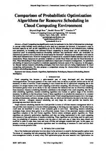
Figure 1. Applied method in this work
solution) and accurate (how close the solution to the global optimum is) performing method in many applications among the already examined methods in the past [11]. Thus, SCE provides a comparative basis for other algorithms that will be presented in this work pertaining to efficiency and accuracy.
2. METHOD Solid fuel consist of long molecules chains. The process of pyrolysis breaks these chains and implies the breakdown into smaller molecules. This process is a requirement of transfer the molecules from the solid into the gas phase. Different material characteristics, like properties thermal conductivity, specific heat or the permeability influence this process. However, the most pyrolysis reaction rates are described by the Arrhenius equation, which expresses the temperature dependence of the physical and chemical reaction. The kinetic constants, activation energy E and pre-exponential factor A, characterize next to the reaction order the Arrhenius equation [6]. These parameters are often unknown but they correlate to the mass loss of a sample while heating it. This can be observed in bench scale tests like thermogravimetric analysis and mass loss calorimetry. Also, there are several models available to simulate pyrolysis [10, 12]. In this work, Fire Dynamic Simulator (FDS) [13] is used. With the output of bench scale tests and pyrolysis models the method shown in figure 1 can be applied. The outputs (e.g. mass loss) of test and simulation are compared. Then, the input parameters of the simulation are systematically altered by an optimization strategy until both outputs satisfy prescribed criteria. 2.1. Bench Scale Tests and Synthetic Data For this work, two different bench scale tests were used. First, a thermogravimetric analysis (TGA) was used to measure the mass loss of a small sample exposed to a constant heating rate. Second, a mass loss cone calorimeter (MLC) was used to measure the mass loss of a sample exposed to a constant heat flux. In figure 2 the sample chamber of a TGA is shown with the specimen holder marked red. 2
pxpx Figure 2. Left: Equipment of the TGA with PU sample (right)
2.1.1. Thermogravimetric Analysis (TGA) The pyrolysis parameters determined by the TGA specify the thermal decomposition of a solid material. In general and in common practice, the temperature dependence of the pyrolysis reaction rate tends to be described by the Arrhenius equation (1) with reaction rate constant (r), pre-exponential factor (A), activation energy (E), universal gas constant (R) and temperature (T ). r = A · e− RT E
(1)
The mass loss data gained from the TGA will be used to infer absolute preexponential factor (A) and activation energy (E) through optimization strategies. To ensure a thermal equilibrium of the sample, the pyrolysis process will be observed likewise for low heating rates (5 K/min). Here, the sample is polyurethane (PU). 2.1.2. Mass Loss Cone Calorimeter (MLC) The thermal properties of materials like density, conductivity, specific heat and emissivity are essential to describe the heating behavior. These properties can be examined by the mass loss calorimeter [19]. MLC is similar to a cone calorimeter without measuring of the heat release rate. Multiple physical processes affect the heating behavior. To include a part of those processes, a sample will be exposed by different irradiances. In this case, applied heat fluxes are 20 kW/m2 , 30 kW/m2 , 40 kW/m2 , 50 kW/m2 and 75 kW/m2 . The examined material is poly(methyl methacrylate) (PMMA). The experiments are conducted with two different background layers, conductor (aluminum) as well as insulator (ceramic wool), to distinguish different heat losses due to conduction properties. 2.1.3. Synthetic Data For the test series with synthetic data, the same model setup as in the TGA series was used. With the input parameters of table 1 for two materials synthetic data was produced with a heating rate of 10 K/min. 2.2. Simulation Model According to the experiments, simulations has to be conducted on a TGA setup and a MLC setup. Both numerical setups are based on the recommended realizations in the FDS User’s Guide [13]. These recommendations were adapted to the reaction and decomposition steps observed in the experiments. Further details are explained later on. 3
Density1 Conductivity1 Specific Heat1 Reference Temperature1 Reference Rate1 Density2 Conductivity2 Specific Heat2 Reference Temperature2 Reference Rate2
ρ1 500 kg/m3 k1 0.2 W/(m·K) c1 1.0 kJ/(kg·K) Tp,1 315 °C rp,1 0.0056 s−1 ρ2 500 kg/m3 k2 0.2 W/(m·K) c2 1.0 kJ/(kg·K) Tp,2 430 °C rp,2 0.0075 s−1
Table 1. Material parameters for generation of a synthetic data set
2.2.1. TGA The pyrolysis model of FDS is based on equation (1) and is extended by the reaction order and the local oxygen volume fraction [13]. For the modeling of the TGA experiment series, the reaction order is fixed to one. A very thin sample (1 mm) is modeled to minimize the influence of the thermal properties and to focus on the pyrolysis process only. Due to a high heat coefficient of the sample, the simulation results are not influenced by the heating behavior. Three decomposition reactions are assumed, which are responsible for a mass loss of 94% of the sample. These boundary conditions are based mainly on the FDS User’s Guides recommended TGA setup and on the results of the experiments. To get the best fitting of modeling results compared to the experimental results for the Arrhenius parameters A and E, the pyrolysis parameters will be varied and the mass loss of the TGA experiments will be compared with the modeling results until the convergence criteria is satisfied. [14] 2.2.2. MLC A modeling approach similar to the TGA’s is used here. However, the thermal properties, like density, specific heat, conductivity and emissivity will be additionally varied to the pyrolysis parameters. This is done because the thickness of the sample and their influence on the modeling results has to be taken into account. The burning rate and the time of ignition are used to compare the modeling results to the experimental ones. Therefore, the mentioned thermal properties, as well as the pyrolysis parameters will be varied per simulation until the best fitting of mass loss of the experiments is reached. Two different approaches are carried out. The first utilizes only one heat flux (50 kW/m2 ), the second uses all mentioned heat fluxes. 2.3. Optimization Process Figure 3 shows the general optimization approach used in this work in a simplified diagram. Firstly, parameters that characterizes thermophysical and pyrolysis material properties were generated as input data for the simulation by a predefined parameter estimation method. Based on these parameters an input file for 4
Start optimization process Estimate Parameters
no
Simulate
Apply fitness function
Convergence?
Check for convergency
yes Output best fitting values Stop optimization process
Figure 3. Optimization process
the simulation is created and the simulation is performed. Then the simulation output data for normalized mass and mass loss rate is compared to experimental data by applying a fitness function. For all algorithms a root-mean-square error function (RMSE) is applied to calculate the fitness. The negation of this value is used to generate a maximization problem. If the calculated fitness satisfies predefined convergence criteria, the optimization process is stopped and the associated input values are displayed. Else, the parameter estimation method generates new input parameters based on the previous simulation for a following evaluation loop until the convergence criteria are satisfied. How these parameters are generated depends on the single parameter estimation method and is described in section 2.4. The decision for an specific optimization algorithm is often not based on performance for a specific problem but on availability for the used framework, computing system and simulation model. Thus, an open source framework was chosen for this work to make the application of the used algorithms publicly available and reproducible, easy to use and capable of parallel computing. The software package the satisfies the above requirements is is an open source python based package called SPOTpy used in version 1.2.25 [5] and for the actual simulation, FDS 6.3.2 [13] was used. Thereby SPOTpy hosts the parameter optimization methods, generates input files for the simulation, calls the simulation, 5
applies the fitness function on the data gained from the simulation and checks for convergence. The simulations for each generation were computed in parallel via Message Passing Interface (MPI) to increase the speed of the algorithms. FDS is used as serial single core version whereas several FDS simulations were computed in parallel. Most simulations were done on the HPC system JURECA at the Jülich Supercomputing Centre (JSC). 2.4. Optimization Algorithms As the ‘No free lunch’ theorem states, there is no optimization algorithm that is most efficient globally. The computational cost, averaged over all problems, is the same for any method [15]. But, for specific problems there are, in fact, more efficient algorithms than others. One way to determine if a algorithm is suitable for a specific class of problems, is to compare its performance the performance of other algorithms on a exemplary problem. Here, two algorithms were selected to be compared to an algorithm (SCE) that is the state of the technology in this field of application. 2.4.1. Shuffled Complex Evolution (SCE) SCE was introduced by Duan for hydrologic model calibration [4]. It combines random and deterministic approaches and uses the concepts of clustering, systematic evolution of a complex of points towards a global improvement and competetive evolution. By this, a local, global and random search takes place. SCE was also widely tested and discussed in application of material data estimation [2, 3] and its process was thoroughly explained on a practical example [9]. Its efficiency and accuracy has been tested against other algorithms and SCE has been stated superior [11]. The basic concept of SCE is to divide a population N into ngs complexes where a local search is done per generation and then compared globally with all complexes. The parallelization in connection with SPOTpy follows equation (2). c = ngs =
N 2 · nopt + 1
(2)
Here, c is the number of used MPI processes, ngs is the number of complexes of SCE, N is the size of population and nopt is the number of parameters to be optimized. In this work, we set ngs =48. 2.4.2. Artificial Bee Colony (ABC) ABC is a swarm intelligence optimization algorithm derived from the foraging behavior of a honey bee swarm [7]. It outperforms frequently used optimization algorithms in standard benchmark tests [8]. Figure 4 shows how ABC works. A Population N is divided into N /2 employed bees and N /2 onlooker bees which both later can become scout bees. Each Bee utilizes a food source xi that has n elements. To initialize the algorithm, for 6
Start ABC
Initialization
Employed bee phase
Onlooker bee phase no Scout bee phase
Convergence? yes
Stop ABC
Figure 4. Flow chart of ABC Algorithm
7
xi,m,0 , where i = 1...N /2 and m = 1...n, an initial solution is produced by equation (3) with lm and um as lower respective upper bound of xi,m . xi,m,0 = lm + rand(0, 1) · (um − lm )
(3)
Then f (xi ) is calculated and a fitness function, in this case RMSE, is applied to generate f it(xi ). In the employed bee phase, a new food source vi in the neighborhood of xi is evaluated. It is generated by equation (4) where t is a random chosen parameter index, Φ a random number in [−a, a], a predefined factor, and xk a random selected food source with k ̸= i. vi,t = xi,t + Φ(xi,t − xk,t )
(4)
Then f (vi ) is calculated and a fitness function, in this case RMSE, is applied to generate f it(vi ) and a greedy selection is applied between f it(xi ) and f it(vi ). The better solution survives and replaces xi . The onlooker bee phase is characterized by an probability distributed assignment based on the probability values calculated by equation (5). The assignment is done by a roulette wheel selection method. So it is more likely that a onlooker bee explores a food source near a food source with a good f (xi ). f it(xi ) pi = ∑N /2 i=1 f it(xi )
(5)
After xi is chosen for a single onlooker bee, vi is calculated by equation (4) and a greedy selection is applied between f it(xi ) and f it(vi ). The better solution survives and replaces xi . If there can’t be found a better fitness in the employed or onlooker phase, after z trials a bee becomes a scout bee and discovers a new random food source. A new random solution is generated by equation (3), where z is a limit that ensures not to get trapped in local extrema with z = N /c with c ∈ {1; 2; 4}. This is called the scout bee phase. These Steps are repeated until a convergence criterion is satisfied. To recap, there are two parameters beside the population/generation ratio to tweak this algorithm. Through all the simulations, it was chosen z = N /4, a = 0.1 and N = 96. Parallelization here is reasonably possible with c = N /2, because the single phases proceed successive. 2.4.3. Fitness Scaled Chaotic Artificial Bee Colony (FSCABC) FSCABC is a modified Version of ABC. It was first introduced for path planning of unmanned combat air vehicles [16] and also successfully used for classifying magnetic resonance brain images [17]. In both cases FSCABC performed significantly better in efficiency and accuracy than all other tested algorithms, including ABC, while SCE was not taken into account. 8
Compared to ABC the enhancements are a changed fitness scaling function and an altered (pseudo) random number generator. The fitness function is shown in equation (6) and is called power rank fitness scaling [18]. rk f it(xi ) = ∑N i
k i=1 ri
(6)
f it(xi ) is used in equation (5) where ri is the rank of the ith individual bee after sorting the bees of the population (which size is N ) ascending by there raw fitness value. k is an exponent, that has to be defined. In this work, we set k = 4. The used (pseudo) random number generator [1] is a chaotic random number generator shown in Equation (7). xn+1 = 4 · xn · (1 − xn )
(7)
Equation (7) with x0 ∈ (0, 1) and x0 ̸∈ {0.25, 0.5, 0.75} produces a chaotic sequence. It is used to generate the random solution in the scout bee phase. Compared to a normal random number generator, x can travel ergodically over the defined space. With this algorithm, it is also z = N /4, a = 0.1. The same rule for parallelization as ABC applies here, too.
3. RESULTS Overall, the three algorithms were compared in four different experimental setups. Two were conducted on a TGA setup, where one was conducted with synthetic data and one with bench scale TGA data, while the other two were conducted on a MLC setup, both using data from bench scale MLC experiments, one with only one heat flux applied and the other one with five different heat fluxes. 3.1. Synthetic data In this case, ten input parameters were determined on a TGA setup with synthetic data as target. For two reactions, parameters density, thermal conductivity, specific heat, reference temperature and reference rate were used each, while the two latter ones characterize A and E. For each algorithm 100000 evaluations where done, each repeated five times to evaluate robustness of the algorithms with the model described in section 2.1.3. In table 2 the best fit (f itbest ) as raw (RMSE) fitness value is shown for each trial and algorithm. Also the number of evaluations (j) after which it was achieved is stated. As can be seen, ABC and FSCABC reach a similar fitness value in all of the five trials while ABC clearly needs more evaluations (factor 1.5…6.2) to reach the same fitting. In this case, SCE is faster than ABC and partly FSCABC but stagnates at a far inferior fit than the other two algorithms. In figure 5 the development of f itbest for all algorithms is shown during trial 4. It can be seen that all three algorithms after 20000 evaluations improve 9
Trial 1 f itbest ABC 0.0442 FSCABC 0.0440 SCE 0.0492
j 69243 35173 11609
Trial 2 f itbest 0.0444 0.0434 0.0571
j 67589 51296 34611
Trial 3 f itbest 0.0439 0.0440 0.0477
j 80906 37980 68659
Trial 4 f itbest 0.0451 0.0440 0.0571
j 94351 15686 51781
Trial 5 f itbest 0.0439 0.0439 0.0504
Table 2. Results of optimization (synthetic data)
Fitness of material parameters (synthetic data)
0.00
ABC FSCABC SCE
0.02 0.04
Fitness
0.06 0.08 0.10 0.12 0.14 0
20000
40000 60000 Evaluation
80000
100000
Figure 5. Fitness evolution during optimization process, trial 4
10
j 62951 41798 28148
Density1 /(kg/m3 ) Conductivity1 /(W/(m·K)) Specific Heat1 /(kJ/(kg·K)) Reference Temperature1 /°C Reference Rate1 /s−1 Density2 /(kg/m3 ) Conductivity2 /(W/(m·K)) Specific Heat2 /(kJ/(kg·K)) Reference Temperature2 /°C Reference Rate2 /s−1
ρ1 k1 c1 Tp,1 rp,1 ρ2 k2 c2 Tp,2 rp,2
Target 500 0.2 1.0 315 0.0056 500 0.2 1.0 430 0.0075
ABC 631 0.269 0.819 320 0.00384 355 1.16 0.871 400 0.0462
FSCABC 400 0.607 1.07 316 0.00478 297 1.67 1.27 400 0.0624
SCE 513 0.950 0.739 399 0.0007101 464 0.946 0.749 238 0.486
l 250 10−4 10−4 100 10−4 250 10−4 10−4 100 10−4
u 750 2 2 500 0.9 750 2 2 500 0.9
Table 3. Results of optimization (synthetic data), trial 4
only a little. FSCABC has achieved the highest fitness with the highest slope, ABC a similar value and SCE a way inferior fitting until then. In table 3 the parameters associated with f itbest are shown. l and u describe the lower and upper bounds, respectively. For material one the values achieved with ABC and FSCABC are remotely close to the target values. All other values are not close to the target values. However, this is nothing a metaheuristic optimization process can provide in the first place, especially if many different solutions generate a similar output, as it is here. The normalized mass against temperature associated with values from table 3 is plotted in figure 6. Graphs of ABC and FSCABC are similar and follow the target closely, whereas the SCE graph represents only the trend of the target function. 3.2. TGA A similar setup is used as in the case before. The target data (normalized mass loss) is gained from a TGA experiment (heating rate 5 K/min) with PU. The pyrolysis is characterized by three reactions with the parameters reference temperature and pyrolysis range for each reaction. Hence, six parameters have to be optimized. As with the synthetic data, here are also 100000 evaluations are conducted and repeated three times for each optimization method. The results are shown in table 4. SCE reaches the same f itbest after at most 29000 evaluations. FSCABC needs between 18000 and 96000 evaluations for the same f itbest . ABC needs at least 54000 evaluations to find a f itbest that is inferior to both, FSCABC and SCE. Figure 7 shows the optimization process of trial 3. FSCABC and SCE are characterized with a similar development, where f itbest of FSCABC rises slightly earlier and SCE achieves a insignificantly better solution in the end. After 10000 evaluations, both improve only marginally. ABC rises significantly slower and achieves a inferior result after 58000 evaluations. 11
Best fit (synthetic data)
1.0
Target ABC FSCABC SCE
Normalized mass
0.8 0.6 0.4 0.2 0.0
100
200
300 400 500 Temperature (°C)
600
700
800
Figure 6. Best fit (synthetic date), trial 4
Trial 1 f itbest ABC 0.4335 FSCABC 0.4177 SCE 0.4175
j 86161 96426 14652
Trial 2 f itbest 0.4300 0.4181 0.4175
j 70716 87020 24736
Trial 3 f itbest 0.4288 0.4179 0.4175
j 57842 76092 29279
Trial 4 f itbest 0.4467 0.4210 0.4175
Table 4. Results of optimization (TGA data)
12
j 54370 17875 22977
Trial 5 f itbest 0.4222 0.4177 0.4175
j 89871 23540 29243
Fitness of material parameters (TGA)
0.0
ABC FSCABC SCE
0.2
Fitness
0.4 0.6 0.8 1.0
0
20000
40000 60000 Evaluation
80000
100000
Figure 7. Fitness evolution during optimization process, trial 3
13
Reference Temperature1 /°C Pyrolysis Range1 /°C Reference Temperature2 /°C Pyrolysis Range2 /°C Reference Temperature3 /°C Pyrolysis Range3 /°C
Tp,1 Tr,1 Tp,2 Tr,2 Tp,3 Tr,3
ABC 275 123 369 88 596 49
FSCABC 279 103 368 98 619 102
SCE 277 99 368 98 625 98
l 250 50 250 50 550 20
u 400 200 450 200 750 200
Table 5. Results of optimization (TGA), trial 3 Trial 1 f itbest ABC 1.2931 FSCABC 1.1402 SCE 1.1391
j 63167 95545 36072
Trial 2 f itbest 1.3272 1.1471 1.1391
j 6955 78981 17250
Trial 3 f itbest 1.2645 1.1405 1.1391
j 16999 68869 18854
Trial 4 f itbest 1.1588 1.1428 1.1390
j 55819 50929 32574
Trial 5 f itbest 1.1626 1.1407 1.1390
j 73290 89018 31724
Table 6. Results of optimization (MLC50 data)
Table 5 shows the corresponding input values for f itbest of trial 3 and the applicated boundary values. As stated before, the values of FSCABC and SCE differ only insignificantly, while the values of ABC differs significantly. Figure 8 shows the normalized mass against time for the target function and the simulations conducted with the parameters from table 5. The graphs for the target function, FSCABC and SCE are hardly distinguishable from each other. Only the graph for ABC is discernable different. 3.3. MLC50 For MLC50 , a MLC setup was used, were a PMMA sample is exposed to a single heat flux (50 kW/m2 ). The decomposition of PMMA is modeled as one reaction, hence there are five parameters to be optimized: density, thermal conductivity, specific heat, reference temperature and pyrolysis range. In table 6, f itbest for each algorithm is shown and when it was achieved. For each algorithm, 100000 evaluations per trial were done for a heat flux of 50 kW/m2 . Like in the previous case, SCE and FSCABC have a very similar f itbest , too. Also, f itbest of SCE is a bit better than f itbest of FSCABC and is reached faster. ABC is inferior in both, efficiency and accuracy. What can be seen in table 6 is shown for trial 1 in figure 9 against the realized evaluations. Even if SCE and FSCABC work totally different, they have almost the same behavior in finding f itbest while ABC needs more evaluations to achieve a comparable f itbest . Table 6 shows the material parameters gained through f itbest of each algorithm. Those of SCE and FSCABC are very similar. Figure 10 shows the normalized mass against time for the target function and the simulations conducted with the parameters from table 5 for all three algorithms with two different background layers each. The graphs for the target 14
Best fit (TGA)
1.0
Target ABC FSCABC SCE
Normalized mass
0.8 0.6 0.4 0.2 0.0
100
200
300 400 Temperature (°C)
500
600
700
Figure 8. Fitness evolution during optimization process, trial 3
Density1 /(kg/m3 ) ρ1 Conductivity1 /(W/(m·K)) k1 Specific Heat1 /(kJ/(kg·K)) c1 Reference Temperature1 /°C Tp,1 Pyrolysis Range1 /°C Tr,1
ABC 1451 0.150 1.631 159 424
FSCABC 1229 0.116 1.936 217 334
SCE 1217 0.117 1.996 217 332
l 1 10−5 10−5 1 1
Table 7. Results of optimization (MLC50 data), trial 1
15
u 10000 1 2 1000 1000
Fitness of material parameters (MLC50 )
0.0
ABC FSCABC SCE
0.5 1.0
Fitness
1.5 2.0 2.5 3.0 3.5 4.0
0
20000
40000 60000 Evaluation
80000
100000
Figure 9. Fitness evolution during optimization process, trial 1
16
Best fit, heating rate: 50 kW/m2
1.0
Target iso Target alu ABC iso ABC alu FSCABC iso FSCABC alu SCE iso SCE alu
Normalized mass
0.8 0.6 0.4 0.2 0.0
0
200
400
600
800 1000 1200 1400 1600 1800 Time (s)
Figure 10. Fitness evolution during optimization process, trial 1
function, FSCABC and SCE are hardly distinguishable from each other. Only the graph for ABC is discernable different. 3.4. MLCall For MLCall , a MLC setup was used, were ten PMMA samples with identical properties are exposed to five heat fluxes (20 kW/m2 , 30 kW/m2 , 40 kW/m2 , 50 kW/m2 and 75 kW/m2 ) with each an isolating and a heat conducting background layer to take into account effects that occur at different heat fluxes. The decomposition of PMMA in this setup is also modeled as one reaction, hence there are five parameters to be optimized: density, thermal conductivity, specific heat, reference temperature and pyrolysis range. For all heat fluxes, 30000 evaluations were carried out for each algorithm with five repetitions. The subsequent f itbest for each algorithm and trial is shown in table 8. It can be observed a similar behavior as in the optimization of MLC50 for f itbest . SCE has the best, FSCABC follows closely and ABC by far. The needed evaluations for f itbest of SCE and FSCABC on the other hand, are both now in the range of 18000 to 29000. Figure 11 shows the development of the optimization for all of the three algorithms of trial 3. Here, FSCABC and SCE are acting very similar again while ABC needs more evaluations to find a proper solution. Table 9 shows the gained 17
Trial 1 f itbest ABC 2.5287 FSCABC 1.3970 SCE 1.3945
j 16486 21627 18351
Trial 2 f itbest 1.8774 1.4096 1.3945
j 48305 26392 14216
Trial 3 f itbest 1.7966 1.4519 1.3945
j 28439 18872 21843
Trial 4 f itbest 1.4523 1.4060 1.3945
j 51624 20584 14326
Trial 5 f itbest 3.0999 1.4498 1.3945
j 12838 28671 26514
Table 8. Results of optimization (MLCall data)
Density1 /(kg/m3 ) ρ1 Conductivity1 /(W/(m·K)) k1 Specific Heat1 /(kJ/(kg·K)) c1 Reference Temperature1 /°C Tp,1 Pyrolysis Range1 /°C Tr,1
ABC 2036 0.217 1.738 205 301
FSCABC 1428 0.131 1.828 228 310
SCE 1192 0.119 1.766 239 336
l 1 10−5 10−5 1 1
u 10000 1 2 1000 1000
Table 9. Results of optimization (MLCall data), trial 3
material parameters and corresponding boundary values. In a plot of normalized mass against time for the target function and f itbest of all algorithms, the graphs are indistinguishable as in the plot of MLC50 , so this plot is not shown.
4. CONCLUSION In this work, two optimization algorithms, Artificial Bee Colony and Fitness Scaled Chaotic Artificial Bee Colony, which bases on ABC, were presented in application for material parameter estimation in fire simulation. The performance in accuracy and efficiency of these algorithms is compared to the current standard algorithm SCE with synthetic data and data from bench scale tests in a parallelized computing environment. FSCABC is superior in all test cases to ABC regarding accuracy and efficiency. Even if SCE in most cases found the best solution, the solution of FSCABC is very close to SCE’s solution. It can be stated that the performance of FSCABC is at least very similar to the performance of SCE. Furthermore, it was shown that both, ABC and FSCABC produce robust solutions. In future research it has to be examined, if tweaking parameters of FSCABC like N ,a,k and z can obtain a superior performance.
5. ACKNOWLEDGMENTS The authors gratefully acknowledge the computing time granted (project jjsc27) on the HPC-cluster JURECA Jülich Supercomputing Centre (JSC).
REFERENCES 1. Ranjan Bose, and Amitabha Banerjee. “Implementing Symmetric Cryptography Using Chaos Functions.” In Proceedings of the 7th International Conference on Advanced Computing and Communications, 318–321. Citeseer. 1999.
18
Fitness of material parameters (MLCall )
0.0
ABC FSCABC SCE
0.5 1.0
Fitness
1.5 2.0 2.5 3.0 3.5 4.0
0
5000
10000
15000 Evaluation
20000
25000
30000
Figure 11. Fitness evolution during optimization process, trial 3
19
2. Marcos Chaos, Mohammed M Khan, Niveditha Krishnamoorthy, John L de Ris, and Sergey B Dorofeev. “Evaluation of Optimization Schemes and Determination of Solid Fuel Properties for CFD Fire Models Using Bench-Scale Pyrolysis Tests.” Proceedings of the Combustion Institute 33 (2). Elsevier: 2599–2606. 2011. 3. M Chaos, MM Khan, N Krishnamoorthy, JL De Ris, and SB Dorofeev. “BenchScale Flammability Experiments: Determination of Material Properties Using Pyrolysis Models for Use in CFD Fire Simulations.” In Proceedings of the 12th International Fire Science and Engineering Conference, Interflam2010, Nottingham, UK, 697–708. 2010. 4. QY Duan, Vijai K Gupta, and Soroosh Sorooshian. “Shuffled Complex Evolution Approach for Effective and Efficient Global Minimization.” Journal of Optimization Theory and Applications 76 (3). Springer: 501–521. 1993. 5. Tobias Houska, Philipp Kraft, Alejandro Chamorro-Chavez, and Lutz Breuer. “SPOTting Model Parameters Using a Ready-Made Python Package.” PloS One 10 (12). Public Library of Science: e0145180. 2015. 6. Morgan J Hurley, Daniel T Gottuk, John R Hall Jr, Kazunori Harada, Erica D Kuligowski, Milosh Puchovsky, John M Watts Jr, Christopher J Wieczorek, and others. SFPE Handbook of Fire Protection Engineering. Springer. 2015. 7. Dervis Karaboga. An Idea Based on Honey Bee Swarm for Numerical Optimization. Technical report-tr06, Erciyes university, engineering faculty, computer engineering department. 2005. 8. Dervis Karaboga, and Bahriye Basturk. “A Powerful and Efficient Algorithm for Numerical Function Optimization: Artificial Bee Colony (ABC) Algorithm.” Journal of Global Optimization 39 (3). Springer: 459–471. 2007. 9. Mohammed M. Khan, Archibald Tewarson, and Marcos Chaos. “Combustion Characteristics of Materials and Generation of Fire Products.” In SFPE Handbook of Fire Protection Engineering, edited by Morgan J. Hurley, Daniel T. Gottuk, John R. Hall Jr., Kazunori Harada, Erica D. Kuligowski, Milosh Puchovsky, Jose´ L. Torero, John M. Watts Jr., and CHRISTOPHER J. WIECZOREK, 1143–1232. Springer New York, New York, NY. 2016. doi:10.1007/978-1-4939-2565-0_36. 10. C Lautenberger. “Gpyro-A Generalized Pyrolysis Model for Combustible Solids Users’ Guide (Version 0.650).” University of California, Berkeley. 2008. 11. CHRIS Lautenberger, and AC Fernandez-Pello. “Optimization Algorithms for Material Pyrolysis Property Estimation.” Fire Safety Science 10: 751–764. 2011. 12. Kevin McGrattan, Simo Hostikka, Randall McDermott, Jason Floyd, Craig Weinshenk, and Kristopher James Overholt. Fire Dynamics Simulator Technical Reference Guide Volume 1: Mathematical Model. Apr. 2015. 13. Kevin McGrattan, Simo Hostikka, Randall McDermott, Jason Floyd, Craig Weinshenk, and Kristopher James Overholt. Fire Dynamics Simulator User’s Guide. Apr. 2015. 14. C. Trettin, and Goertz, R., Arnold, L. Wittbecker F.-W. “A Contribution to Pyrolysis Modeling.” Interflam 2016, Windsor. 2016. 15. D Wolpert, and W Macready. “No Free Lunch Theorems for Search (Technical Report Sf IT R-95-02-010).” Santa Fe Institute, Santa Fe, NM. 1995. 16. Yudong Zhang, Lenan Wu, and Shuihua Wang. “UCAV Path Planning Based on FSCABC.” Inf-an Int Interdiscip J 14 (3): 687–692. 2011. 17. Yudong Zhang, Lenan Wu, and Shuihua Wang. “Magnetic Resonance Brain Image Classification by an Improved Artificial Bee Colony Algorithm.” Progress In Electromagnetics Research 116. EMW Publishing: 65–79. 2011.
20
18. Yudong Zhang, Lenan Wu, and Shuihua Wang. “UCAV Path Planning by FitnessScaling Adaptive Chaotic Particle Swarm Optimization.” Mathematical Problems in Engineering 2013. Hindawi Publishing Corporation. 2013. 19. “Mass Loss Calorimeter [online].” Web Page. 2016. http://www.fire-testing. com/mass-loss-calorimeter.
21