of Hazard-free Circuits from Signal Transition Graphs. Enric Pastor and ...... LMBSV92] Luciano Lavagno, Cho W. Moon, Robert K. Brayton, and A. Sangiovanni-.
Polynomial Algorithms for Complete State Coding and Synthesis of Hazard-free Circuits from Signal Transition Graphs Enric Pastor and Jordi Cortadella UPC/DAC Report No. RR-93/17 September 1993
This work has been supported by the Ministry of Education of Spain (CICYT) under contract TIC 91-1036, Dept. d'Ensenyament of Generalitat de Catalunya, and ACiD-WG (Esprit 7225).
Polynomial Algorithms for Complete State Coding and Synthesis of Hazard-free Circuits from Signal Transition Graphs Enric Pastor and Jordi Cortadella Department of Computer Architecture Universitat Polit�ecnica de Catalunya
Abstract
Methods for the synthesis of asynchronous circuits from Signal Transition Graphs (STGs) have commonly used the State Graph to solve the two main steps of this process: the state assignment problem and the generation of hazard-free logic. The size of the State Graph can be of order O(2n ), where n is the number of signals of the circuit. As synthesis tools for asynchronous systems start to mature, the size of the STGs increases and the exponential algorithms that work on the State Graph become obsolete. This paper presents alternative algorithms that work in polynomial time and, therefore, avoid the generation of the SG. With the proposed algorithms, STGs can be synthesized and hazard-free circuits generated in extremely low CPU times. Improvements in 2 or 3 orders of magnitude (from hours to seconds) with respect to existing algorithms are achieved when synthesizing fairly large STGs.
1 Introduction Asynchronous circuits have gained interest in the last few years, specially in the area of interface circuits. However they have not been widely used due to the di�culty of design and the lack of synthesis and veri cation tools. Signal Transition Graphs (STGs) have been proposed as a speci cation formalism for asynchronous control circuits [RY85, Chu86]. Several synthesis approaches from STGs have been proposed under di�erent types of assumptions on the structure of the STG (marked graph, free-choice net), the mode of operation of the circuit (fundamental mode, single/multiple input change conditions), and the delay model for the components of the circuits (unbounded/bounded gate/wire-delay models, pure/inertial gate delay). Most current designs based on STG speci cations have been handcrafted and, therefore, their complexity is relatively manageable by designers. Even for some of such descriptions, the synthesis algorithms take a signi cant CPU time, of the order of several minutes or hours. This results directly from the fact that the number of states derived from an STG rapidly exploits with the number of signals and the degree of parallelism intrinsic to the underlying net. Similarly to what happened with synchronous FSMs, as high-level synthesis tools start becoming mature, asynchronous FSMs will be automatically generated to specify the behavior of interface and data-path controllers [CB92] and its complexity will be no longer manageable by exponential algorithms. 1
Therefore, there is a need to devise algorithms whose complexity depends on the size of the description rather than in the number of states. This paper aims at making some key contributions in this direction. The algorithms proposed must, rst, avoid the enumeration of the states generated by the STG description and then, avoid net traversals that depend on the number of states of the STG. In this way, polynomial algorithms are proposed. Algorithms for the two key problems involved in the synthesis from STGs are discussed: � The Complete State Coding problem: An algorithm for Free-choice nets with multiple transitions is presented. � The synthesis of a hazard-free circuit : An algorithm is presented for the generation of a speed-independent two-level logic circuit operating in fundamental mode and multiple input-change conditions. The assumption of fundamental mode with multiple input changes (or burst mode [YDN92]) has resulted to be realistic for numerous designs but it is not applicable to any speci cation in general. The other assumption, speed-independence (or unbounded gate-delay model), considers that wires have zero delay whereas gate delays have no bounds. Speed-independence is equivalent to delay-insensivity under the assumption that forks are isochronic [vB92]. The two-level circuits generated by the proposed polynomial algorithms can be valid implementations of the input speci cations if the environment behaves as assumed by the operation mode. Furthermore, this implementation can be transformed into a multi-level logic circuit with more restrictive delay models by using existing techniques [LMBSV92].
1.1 Previous Work
Methods for solving the CSC problem in STGs have been proposed in [Van90, LMBSV92, VLGM92, YCLGM93]. Vanbekbergen [Van90] and Ykman [YCLGM93] have presented algorithms that work directly on the STG, but only in [Van90] a polynomial-time technique based on the lock graph theory has been proposed. However, this technique is only applicable to marked graphs with single transitions. The other approaches require the construction of the State Graph (SG), which can have a number of states of O(2n ), being n the number of signals. Among the techniques proposed for hazard-free synthesis, we will mention some of the most relevant in the area of asynchronous circuits. Nowick and Dill [ND91] guarantee hazard-free implementations of asynchronous FSMs by using local clocking in the circuit. Yun et al. [YDN92] present 3D state machines in which synthesis and hazard analysis is based on the construction of a three-dimensional next-state table. Nowick and Dill also present in [ND92] a QuineMcCluskey-based method to generate two-level hazard-free logic. Kung presents in [Kun92] a set of optimization algorithms for multi-level synthesis that maintain the hazard-freeness of the original implementation. In the area of STGs, algorithms for hazard-free synthesis have been proposed by Chu [Chu92], Moon et al. [MSB91], and Lavagno et al. [LKSV91, LMBSV92] assuming di�erent delay models and modes of operation. The most restrictive delay model (bounded wire delay) has been considered in [LMBSV92] where hazards are eliminated by solving a linear programming problem. 2
However, all the proposed approaches require an exhaustive analysis of the states of the system either at the level of State Graph or next-state tables and, therefore, their corresponding algorithms are exponential.
2 De nitions This section presents the basic de nitions and notations used along the paper. Special care has been taken to be consistent with the notation used by other authors [Mur89, Chu87, Hac72, Van90, LMBSV92, BHMSV84].
2.1 Petri Nets
A Petri net is a 4-tuple hP ; T ; F ; moi, where P is a set of places, T is a set of transitions, F � (P�T ) [ (T � P ), such that dom(F ) [ range(F ) = P [ T , is the ow relation, and mo is the initial marking. We use the following symbols to de ne the pre- and post-set of every place p or transition t: �t = fp : (p; t) 2 Fg � the set of input places of t t� = fp : (t; p) 2 Fg � the set of output places of t �p = ft : (t; p) 2 Fg � the set of input transitions of p p� = ft : (p; t) 2 Fg � the set of output transitions of p
There are some subclasses of Petri nets that are relevant to the goal of this paper, i.e. State Machines and Free-choice nets .
De nition 1 [Mur89] A State Machine (SM) is a Petri net such that each transition t has exactly one input place and one output place. i.e.,
8t 2 T : j �t j=j t� j= 1
De nition 2 [Mur89] A Marked Graph (MG) is a Petri net such that each place p has exactly one input transition and exactly one output transition, i.e., 8p 2 P : j �p j=j p� j= 1
De nition 3 [Mur89] A Free-choice net (FC net) is a Petri net such that every arc from a place is either a unique outgoing arc or a unique incoming arc to a transition.
8p 2 P : j p� j� 1 _ �(p�) = fpg
3
2.1.1 Petri Net Behavior
A marking m of a Petri net is a function m : P ! Z + , that assigns to each place a non-negative integer. A place pi 2 P with marking m contains m(pi ) tokens. A transition t is enabled in a marking m (denoted m[ti) when all its predecessor places are marked with at least one token. When an enabled transition in marking m1 res, a token is removed from every predecessor place and a token is added to every successor place, reaching a marking m2 . This is denoted by m1[tim2. A marking mn is said to be reachable from a marking mo ([mo imn ) if there is a sequence of rings that transforms mo into mn , and will be noted as [mo imn . The set of all markings reachable from mo is denoted by [mo i. A Petri net is said to be live if every transition can be enabled through some sequence of rings from the initial marking mo . A Petri net is safe if no place can ever be assigned more than one token after any sequence of rings from the initial marking mo . De nition 4 [Mur89] An FC net is live if every transition can be enabled through some sequence of rings from the initial marking mo . De nition 5 [Mur89] An FC net is safe if no place can ever be assigned more than one token after any sequence of rings from the initial marking mo . [Hac72] proved that a live and safe FC net can be decomposed into sets of SM-components (SMCs) that cover the net. Lemma 6 [Hac72] A live and safe FC net is covered by strongly-connected SMCs each of which has exactly one token at any marking mn 2 mo [i.
2.2 Signal Transition Graph
Signal Transition Graphs (STGs) are Petri nets, whose transitions are interpreted as value changes on input, output and internal signals of the circuit. Rising and falling transitions for signal t are denoted by t+ and t? respectively. The following notation will be used: � ti denotes a signal in the STG. � t�i denotes an up- or down-transition of signal ti . � t�i is a complementary transition of t�i , t�i = t+i ) t�i = t?i and t�i = t?i ) t�i = t+i . � Sa denotes the set of all signals in the STG. SNI denotes the set of non-input signals. De nition 7 [LMBSV92] An STG is live if: 1. the underlying FC net is live and safe, and 2. for each signal ti there is at least one SMC, initially marked with exactly one token, such that: � it contains all transitions t�i of signal ti. � each path from a transition t�i to another transition t�i contains also a complementary transition t�i .
4
2.3 State Graph
The State Graph (SG) of an STG is a Finite Automata in which the states correspond to markings of the STG. An edge labeled with t and going from state s1 (corresponding to marking m1) to state s2 (corresponding to marking m2) indicates that m2 can be reached from m1 after ring transition t. Synthesis procedures based on STGs [Van90, MSB91, LKSV91] use the signals of the circuit as state variables. If the STG is live, each state (marking) si of the SG is assigned a binary vector of signal values (state code). The following notation will be used: � vi 2 f0; 1gn (n = jSaj) is the code of state si . � vij denotes the value of signal tj in the state si . c = fv1; : : :; vn g denotes the � If M = fm1; : : :; mng is a set of markings of an STG, then M set of state codes of the SG corresponding to the markings in M .
Ri+ Ri+ p0
p2
p0
Ri-
Ri+ p2
Ro+ p1
p3
Ai+
p7
p0
Ri-
Ro+ p3
p5
AiRo-
(a)
p6
p1
SM0
Ai-
Ai+ p4
Ro+
Ro-
p4 p4
p7
Ai+
p5
SM1 (b)
Ro-
SM2
p6
set of vertices where f evaluates to 0 is the o�-set, and the set of vertices where f evaluates to � is the dc-set. A literal is either a variable or its complement. A cube is a set of literals. Each cube is in correspondence with a set of vertices in f0; 1gn. A cube is called an implicant of a logic function f if it covers some vertex in the on-set and does not cover any o�-set vertex. The Hamming distance between two cubes ci and cj , denoted by d(ci; cj ), is the cardinality of the set of variables xi such that either xi 2 ci and xi 2 cj or xi 2 cj and xi 2 ci . An on-set cover F of a logic function f is a set of cubes such that each cube of F is an implicant of f and each minterm of f is covered by at least one cube of F . An o�-set cover R o� a logic function f , is a cover of the complement of f . We refer the reader to the existing literature on logic synthesis, such as [BHMSV84], to become familiar with the aforementioned nomenclature.
2.5 Next State function and Complete State Coding
If the STG is live, the non-input signals of the circuit can be used directly as state variables, and the next-state function for each signal can be derived from the SG. The next procedure derives the next-state function of a non-input signal ti [Chu87]: Procedure 1 : t
f
t
Let i be a non-input signal and i the next-state function of signal i . of the SG and j the state code of j . For each state j of the SG do:
v
(a) if there is an edge
(d) for all
vj
t?
sj ?! sk fi (vj ) = vji
(b) if there is an edge (c) otherwise let
t+i
sj ?! sk i
s
s
then let
fi (vj ) = 1
then let
fi (vj ) = 0
without a corresponding state in the SG
fi (vj ) = ?
Let
sj
be a state
(don't care)
The next-state function fi , de ned by the above procedure, is said to be well-de ned if for each state code vj , fi is uniquely de ned, i.e. there are not two states sj and sk with the same code (vj = vk ) such that fi (vj ) 6= fi (vk ). If the next-state function is well-de ned for all output signals, then the STG is said to have the Complete State Coding (CSC) property. CSC is a necessary and su�cient condition for a live STG to derive a race-free circuit [MSB91].
De nition 8 A State Graph is said to satisfy a Complete State Coding (CSC) property if, when the same code is assigned to two di�erent states, the transitions of the non-input signals enabled in both states are identical. Figure 2 shows the CSC con icts in the State Graph of the example. For instance, states s1 and s5 have both the same code (v1 = v5 = 110). s1 has no enabled Ro transitions whereas Ro+ is enabled in s5 . Therefore, the STG has not the CSC property. If we derive the next-state function fRo by using procedure 1 we will obtain fRo (v1) = 0 for state s1 and fRo (v5) = 1 for state s5 . CSC con icts also exist for the pairs of states (s7 ,s9 ), (s2 ,s6 ), and (s10 ,s12). 6
Ai-
s1 110 Ri-
RiAi-
s3 010 Ri+
Ri Ai Ro
s4 000
Ri+
s5 110
Ai-
Ro+ s7 111
s2 100
s6 100
Ro+ Ai-
s8 Ai+ 101
Ros9 111
Ri-
Ri-
Ri-
s10 Ai011
s11 Ai+ 001
s12 011
Ro-
implementation which is hazard-free under the Multiple Signal Change condition.
4 A Polynomial Algorithm to Solve the CSC Problem As shown before, the analysis of the CSC property can be done at the SG level. Most algorithms proposed so far to solve the state assignment problem operate on the SG [LMBSV92, VLGM92]. Previous works based on lock relations [YCLGM93, LL92] operate directly on the STG. However, the approach presented in [YCLGM93] is restricted to marked graphs and shows an exponential worst-case complexity. [LL92] can be applied to FC-STGs but also has an exponential worst case. Next we present a novel approach to verify the CSC property for FC-STGs. It operates on the STG and has polynomial complexity.
4.1 Exponential-time CSC Veri cation
De nition 9 Given an STG S and a non-input signal ti, we de ne M+i = fmj 2 [m0i j 9t+i : mj [t+i ig M1i = fmj 2 [m0i j vji = 1 ^ 6 9t?i : mj [t?i ig M?i = fmj 2 [m0i j 9t?i : mj [t?i ig M0i = fmj 2 [m0i j vji = 0 ^ 6 9t+i : mj [t+i ig M+i (M?i ) is the set of markings in which some t+i (t?i ) is enabled. M1i (M0i ) is the set of markings in which the corresponding state code is such that vji = 1 (vji = 0) and no t�i transition
is enabled. Given the non-input signal Ro of the example (see Figure 2), Table 1 shows its Mi sets. M+Ro (M?Ro ) is the set of all markings where raise (fall) transitions of the signal Ro are enabled, fm5,m6g for M+Ro and fm9,m12g for M?Ro . M1i (M0i ) is the set of markings where signal Ro equals 1 (0) and no falling (raising) transitions of Ro are enabled, fm7,m8,m10,m11g for M1i and fm1,m2,m3,m4g for M0i . There is an exact implication between the CSC property de nition and the Mi sets for the non-input signals of the STG. This implication allows checking the CSC property by intersecting some of this sets M+i .
c+Ro = f110; 100g M c?Ro = f111; 011g M c1Ro = f111; 101; 011; 001g M c0Ro = f110; 100; 010; 000g M
M+Ro = fm5; m6g M?Ro = fm9; m12g M1Ro = fm7; m8; m10; m11g M0Ro = fm1; m2; m3; m4g
ci sets for signal Ro Table 1: Mi and M 8
Theorem 10 The following statements are equivalent: (a) An STG S has the CSC property c+i \ M c0i = ; ^ M c?i \ M c1i = ; (b) 8ti 2 SNI M Proof: We will prove that :a ) :b and :b ) :a. :a ) :b : If S does not have the CSC property then (from De nition 8) there are two markings m1 and m2 whose corresponding states have the same code and there is a non-input signal ti such that t�i is enabled in m1 and t�i is not enabled in m2. Let us assume that t�i = t+i (the same applies for t�i = t?i ). Since t+i is enabled in m1 then v1i = 0 and m1 2 M+i . Furthermore, v2i = v1i = 0 and no t?i can be enabled in m2 (otherwise v2i = 1). Therefore m2 2 M0i and since c+i \ M c0i 6= ;. m1 and m2 have the same state code, then M + 0 ci \ M ci 6= ; (the same applies for M c?i \ M c1i 6= ;). Then there :b ) :a : Let us assume that M is a non-input signal ti and there are two markings m1 2 M+i and m2 2 M0i with the same code (v1 = v2). Therefore, m1 has an output t+i transition whereas m2 does not have any output t�i transitions and, therefore, S does not have the CSC property. 2 ci sets for the non-input signal Ro . See, for example, that the CSC Table 1 shows the M c0Ro . c+Ro \ M con icts for the states (m1; m5) and (m2; m6) are detected when calculating M The calculation of the Mi sets requires a complete reachability analysis of the net. The ci sets. approach we propose avoids the exponentiality of this analysis by overestimating the M
c i Sets 4.2 Overestimates of the M
De nition 11 For each place p and transition t of an STG, we de ne Vp = fmj 2 [moi j mj (p) = 1g (set of markings with a token in p) Vt = fmj 2 [moi j mj [tig (set of markings in which t is enabled) De nition 12 Let S be a live STG and pi a place. We de ne conc(pi), the set of concurrent places and transitions with respect to pi , as follows:
conc(pi) = ft 2 T j 9mn 2 mo[i s.t. mn [ti ^ mn(pi) = 1 ^ t 62 p�i g [ fp 2 P j p 2 (�t [ t�) for some t 2 conc(pi)g conc(pi) can be calculated in polynomial time for free-choice nets by using the algorithm pre-
sented in Appendix B.
De nition 13 Given a place p and a transition t, we de ne Cp and Ct as the smallest cubes that cover Vbp and Vbt respectively. Vbp can be considered as a set of minterms of jSaj variables. Instead of calculating Vbp by means of a reachability analysis of the net, we propose to calculate an overestimation of Vbp by using the conc(pi) relation. i
i
i
9
Given a place pi , the cube Cpi covers all the binary vectors in Vbpi , and Cpji is the j ? th component of Cpi , corresponding to the signal tj . If no transitions of the signal tj are concurrent with the place pi , then all the binary vectors v 2 Vbpi will be either v j = 1 or v j = 0 and consequently Cpji = v j . To determine the value of Cpji , we must nd the rst transition t�j enabled after ring some transitions from a marking mp where place pi is marked. If t�j is a rising transition then Cpji = 0, otherwise Cpji = 1. If any transition of signal tj is concurrent with pi , then Vbpi will have some binary vectors with v j = 1 and the rest with v j = 0, and therefore Cpji = ?. Given a transition t�i , the cube Cpi covers all the binary vectors in Vbt�i , and it is calculated intersecting the cubes of all its input places. Cp and Ct can be calculated in polynomial time for free-choice nets by using the O(jPj jT j2) algorithm presented in Appendix D. Tables 2 and 3 show the V sets and their corresponding cubes for the example of the PLA interface circuit.
p
Vp
p0 fm5, m6g p1 fm1, m2, m7, m8, m9g p2 fm3, m4, m10, m11, m12g p3 fm7, m8, m10, m11g p4 fm9, m12g p5 fm1, m2, m3, m4g p6 fm1, m3, m5, m7, m10g p7 fm2, m4, m6, m8, m11g
Cp (RiAiRo) 1-0 1-0---1 -11 --0 -1-0-
Table 2: Vp and Cp for the places of the PLA interface circuit
t
Vt
Ri+ fm3, m4g Ro+ fm5, m6g Ri- fm1, m2, m7, m8, m9g Ai+ fm8, m11g Rofm9, m12g Ai- fm1, m3, m5, m7, m10g
Ct (RiAiRo) 0-0 1-0 1--01 -11 -1-
Table 3: Vt and Ct for the transitions of the PLA interface circuit
De nition 14 A set of SMCs, � = fSig, is an SM-cover of an STG S if all members of � are
SMCs of S and all the places and transitions of S are covered by some Si . An SM-cover � is irredundant if no subset of � is an SM-cover.
10
It is easy to prove that for Free-choice nets, an SM-cover also covers all the arcs of the net. Finding an SMC that covers a place or a transition can be done in polynomial time by using the extension of Hack's algorithm [Hac72] presented in Appendix C. Finding an irredundant cover can be done by iterative generation of SMCs that cover places or transitions not covered by previous SMCs. The following algorithm makes a conservative veri cation of the CSC property, i.e. if a CSC con ict exists then it is detected by the algorithm. On the other hand, the use of the C cubes instead of the M sets may produce the detection of non-existing con icts as \potential con icts" and therefore, state disambiguation will be required for those cases.
Procedure 2
has csc property (S) f Let
1 2 3 4 5
g
� = fSm g
be an irredundant SM-cover of S
foreach Sm 2 � do foreach pair of places pj and pk covered by Sm such that j > k do foreach non-input signal ti do if (9t�i 2 p�j ) and (Cp \ Ct� 6= ;) then return false; if (9t�i 2 p�k) and (Cp \ Ct� 6= ;) then return false; return true; k
i
j
i
Theorem 15 An STG S does not have the CSC property =) has csc property(S ) returns false
Proof: If S does not have the CSC property then there are two markings, m1 and m2 , with the same code (v1 = v2 ) and a signal ti such that m1 2 M0i and m2 2 M+i (the same applies for M1i and M?i ). Therefore, there is a transition t�i such that v2 v Ct�i and there is a place pj 2 � t�i such that m1(pj ) = 0 (otherwise m1 2 M+i ). Let Sm 2 � be an SMC that covers pj and t�i (Sm always exists). Then there is a place pk covered by Sm such that m1(pk ) = 1 and, therefore, v1 v Cpk . Thus the con ict is detected because Cpk \ Ct�i 6= ;. 2
4.3 Insertion of State Signals
In order to solve the CSC con icts detected by Procedure 2, state signal transitions are inserted at some of the SMCs of the SM-cover �. First, a Con ict Graph for each Sm 2 � is built.
De nition 16 For each Sm 2 � we de ne the Con ict Graph CG(Sm) as the pair < P ; U >, where P is the set of places of Si and U � (P � P ) is the CSC con ict relation, de ned as follows:
(pi; pj ) 2 U , 9ti 2 SNI s.t. ((9t�i 2 p�i ^ Ct�i \ Cpj 6= ;) _ (9t�i 2 p�j ^ Ct�i \ Cpi 6= ;)).
U contains an edge for each CSC con ict detectable by Procedure 2. Figure 3 depicts the CSC con icts in the SM-cover of the PLA interface circuit. However, the information given by all the CGs is redundant, as it is shown by the following theorem. 11
Theorem 17 Let � be an SM-cover of the STG S . Let us assume that place pj is covered by two SMCs of �. If a CSC con ict between markings m1 and m2 can be detected by means of pj in one of the SMCs, then the same con ict will be detected by means of pj in the other SMC.
Proof: If m1 and m2 have a con ict then v1 = v2 . Let us assume that m1 2 M+i and m2 2 M0i . This con ict can be detected by using the place pj and the SMC Si that covers signal ti , since 9t+i 2 p�j s.t. m1(pj ) = 1 and m2(pj ) = 0, and there is a place pk covered by Si such that pk 62 �t+i and m1(pk ) = 0 and m2 (pk ) = 1. If any other SMC Sj covers the place pj , then Sj also covers t+i and a place pl 62 � t+i such that m1 (pl) = 0 and m2(pl ) = 1. Therefore, v1 v Ct+i 2 and v2 v Cpl , and the CSC con ict is detected in Sj (Ct+i \ Cpl 6= ;).
Ri+
CSC conflict CSC conflict eliminated after redundacy reduction
p0
Ri+
Ro+
p2
p7
Ai+
p3
p0
Ai+
Ri-
Ai-
p4
Ro+ p4 p1
Ro-
p6
Ro-
p5
SM0
SM1
SM2
typical problem of nding a minimum cover . The heuristics used to select the SMCs for con ict disambiguation attempt to iteratively include those SMCs that cover the maximum number of con icts not covered yet by other SMCs. Given an SMC with CSC con icts, pairs of (s+; s?) transitions of a new state signal are inserted, thus partitioning the places covered by the SMC into two sets: the 1-set and the 0-set. The 1-set (0-set) of an SMC with respect to the inserted signal s is the set of places that are located between a rising (falling) and a falling (rising) transition of s. A CSC con ict can then be disambiguated by inserting a state signal in such a way that each of the involved places is located in a di�erent set. Moreover, the same signal can be used to disambiguate multiple con icts at the same time.
1-set
0-set
s+
s-
s+
s-
s+
s+ p8
Ri+ p2
Ri-
RiAi-
s3 0100
s+
Ro+
p3
s+
p7
Ri+ Ai-
p4 p5
Ai+
Ai-
Ro-
(a)
p5
(b)
s7 1111
p4
p6
Ri-
Ro-
s6
1101
p9
1001
Ro+
Ai+
0001
Ri+
s-
s5 p9
Ri Ai Ro s
s13 Ai- s14
p3
s-
s4 0000
0101
p1
1000
Ri-
p0
Ro+
s2
1100
Ri+
p0
Ai-
s1
p8
Ro+ Ai-
0011
Ro-
s15 Ai+
1011
1010
Ri-
s10 Ai- s11 0111
s-
s8
Ri-
s-
s9 1110
Ri-
s16 Ai+ s12 0010
(c)
0110
Ro-
if for any ti 2 SNI there is an Si 2 � such that all transitions of signal ti are covered by Si .
From now on, we will denote by Si an SMC that covers all transitions of signal ti 1 . Figure 5(a) shows the PLA interface circuit after the internal signal insertion, while Figure 5(b) shows the SMC that covers all the non-input signals Ro and s. Figure 5(c) shows the State Graph for the encoded STG, and the recalculated V sets and cubes are presented in tables 4 and 5.
p
Vp
p0 fm5 m6g p1 fm1, m2, m7, m8, m9, m15g p2 fm3, m4, m10, m11, m12, m16g p3 fm7, m8, m10, m11g p4 fm9, m12g p5 fm1, m2, m3, m4g p6 fm1, m3, m5, m7, m10, m13g p7 fm2, m4, m6, m8, m11, m14g pc1 fm13, m14g pc2 fm15, m16g
Cp (RiAiRos) 1-01 1--0----11 -110 --00 -1--0-0-01 -010
Table 4: Vp and Cp for the places of the encoded PLA Interface Circuit
t
Vt
Ri+ fm13 m14g Ro+ fm5, m6g Rifm1, m2, m7, m8, m9, m15g Ai + fm15, m16g Rofm9, m12g Ai- fm1, m3, m5, m7, m10, m13g s+ fm3, m4g sfm8, m11g
Ct (RiAiRos) 0-01 1-01 1---010 -110 -1-0-00 -011
Table 5: Vt and Ct for the transitions of the encoded PLA Interface Circuit
1 Note that one SMC can cover more than one signal
15
5.1 Deriving Logic from a State Machine
We will denote by Fi and Ri the on-set and o�-set covers derived for the next-state function of the non-input signal ti . The on-set and the o�-set of the next-state function fi can be expressed ci sets: in terms of the M c+i [ M c1i On-set(fi ) = M c?i [ M c0i O�-set(fi ) = M Instead, we calculate covers by using the cubes Cp and Ct�i for all places and transitions of signal ti of Si. Given an SMC Si that covers signal ti, the places covered by Si can be partitioned into four sets:
fplaces between a t+i and a t?i transitions and not predecessor of any t?i transitiong fplaces between a t?i and a t+i transitions and not predecessor of any t+i transitiong fplaces predecessor of a t+i transitiong fplaces predecessor of a t?i transitiong Clearly, the state codes of the markings that have a token in some place belonging to Pi1 belong to the on-set of fi . These codes belong to the corresponding Vbp sets and are covered by the corresponding Cp cubes. The state codes belonging to Vbt+ for any rising transition of ti belong to the on-set of fi . These codes are covered by the corresponding Ct+ . Finally, the state codes belonging to Vbp ? Vbt? for any p 2 Pi? and predecessor of t?i belong to the on-set of fi . These codes are also covered by D = Cp ? Ct? . Note that D is not a cube, Pi1 Pi0 Pi+ Pi?
= = = =
i
i
i
i
but a cover. Its calculation can be done in polynomial time as shown in appendix E. The fact that D covers Vbp ? Vbt?i results from the CSC veri cation procedure of the previous section and can be easily proved similarly to theorem 15. We will skip this proof here. This is the reason why the synthesis approach we propose requires the CSC veri cation described by Procedure 2. Thus, an initial Fi cover can be obtained by using this approach (similarly for an initial Ri cover). For hazard elimination, consensus between cubes corresponding to pairs of adjacent places (separated by one transition) and pairs of adjacent places and transitions are properly added. Finally, a prime cover is obtained by expanding the resulting cubes in Fi against Ri.
FRo RRo Fs Rs
CR+ [ Cp3 [ Cp 2 [ (Cp4 ? CR? )[ RiR0o s + Ros + A0i Ros0 (CR+ Cp3 ) [ (Cp3 Cp 2 ) [ (Cp 2 (Cp4 ? CR? )) +Ri s + A0i Ro CR? [ Cp5 [ Cp 1 [ (Cp0 ? CR+ )[ Ai Ro s0 + R0os0 + R0iR0o s 0 0 Cs+ [ Cp 1 [ Cp0 [ (Cp3 ? Cs? ) Ri Ros0 + R0iR0os + Ri R0os + A0i R0o s0 (Cs+ Cp 1 ) [ (Cp 1 Cp0 ) [ (Cp0 (Cp3 ? Cs? )) +R0i R0o + R0o s + RiAi s 0 Cs? [ Cp 2 [ Cp4 [ (Cp5 ? Cs+ ) Ai Ros + A0i Ros0 + Ai Ro s0 + RiR0os0 c
o
c
o
c
o
o
c
o
o
c
c
c
c
Table 6: F and R covers for signals Ro and s ( stands for consensus) 16
Procedure 3 obtains a hazard-free cover Fi for fi .
Procedure 3 hazard-free SOP implementation f
1
foreach non-input signal ti do let Si be an Fi = R i = ;
SMC that covers signal
/* Calculate an initial cover for
2 3
foreach place ?pj covered by Si do if ( 9t = ti 2 +p�j ) Dp = Cp ? Ct elseif ( 9t = ti 2 p�j ) Dp = Ct else Dp = Cp
ti
Fi
*/
Ri
*/
j
j
j
4
j
j
Fi = Fi [ Dp
j
/* Calculate an initial cover for ... Similarly to i ...
F
5
9
g
/* Add consensus for hazard elimination */ covered by i let k be the place in the inset of covered by let l be the place in the outset of covered by i i Consensus pk pl /* if some contains more than one cube, consensus is generated for all cubes */
foreach transition t p p F =F [
D
Fi = expand(Fi ; Ri) /* Fi is expanded
S
do
(D ; D )
t t
Si Si
R
against i, and cubes included in other cubes are eliminated */
Table 6 presents the F and R covers calculated by Procedure 3 before expanding F against R. The nal result of the synthesis is:
FRo = Ros + Ris + A0iRo Fs = R0os + Ai s + R0iR0o Figures 6 and 7 present the nal implemetations for signals s and Ro respectively.
Theorem 19 The Fi and Ri covers obtained by Procedure 3 are valid on-set and o�-set covers
of fi ,i.e. every on-set (o�-set) vertex and no o�-set (on-set) vertex of fi is covered by a cube in Fi (Ri). c sets) to calculate Proof: Procedure 3 uses overestimates of the Vb sets (and consequently of the M Fi and Ri. Therefore, Fi and Ri cover all the on-set and o�-set vertices of fi respectively. Let us prove that Fi and Ri do not intersect by considering all possible intersections between pairs of cubes of Fi (cF ) and Ri (cR). Let us consider that cF and cR have been obtained
17
Ro s 00
01
11
10
00
10
10
01
01
01
10
10
1
0
11
0
1
1
0
10
0
1
01
01
Ri Ai
= oR’ os s++AR FFsRo =R i si s++RA i’i’RR o’o
Ai R s R so Ro Ri
transition cube for T , as follows:
CTj
=
(
? if some t�j 2 T v1j otherwise
Since T is a set of concurrent transitions (they can be red in any order), all states covered by CT are valid states of the SG. Let us assume we are deriving logic for signal ti by using the SMC Si according to Procedure 3. 0 ) 0 transitions. All states covered by CT belong to the o�-set of fi . Therefore, no cube of Fi covers any of them, otherwise the STG would not have the CSC property. Hence, no 1-hazards can be produced. 0 ) 1 transitions. All states covered by CT belong to the o�-set of fi , excepting s2 . Therefore, there is at least one cube of Fi that covers s2 and no cube of Fi that covers the rest of states covered by CT , otherwise the STG would not have the CSC property. Hence, no hazards can be produced. 1 ) 1 transitions. Let us call m1 and m2 the markings corresponding to states s1 and s2 . There is a place p1 covered by Si such that m1(p1 ) = 1. Let us call t the transition in the outset of p1 covered by Si . If t 62 T then CT is completely covered by Cp1 and no 0-hazards can be produced. If t 2 T , let us call p2 the place in the outset of t covered by Si . Hence m2 (p2) = 1. According to Procedure 3, CT will be covered by Cp1 [ Cp2 . Since CT is a cube, then CT is completely covered by the consensus(Cp1 ; Cp2 ) and thus no 0-hazards can be produced. 1 ) 0 transitions. We will prove this case, without loss of generality, by means of the example shown in Figure 8. State s2 (with code v2 ) is the one in which t?i is enabled. t+1 , t+2 , and t+3 are the the set of concurrent transitions T . Procedure 3 will include the following cubes to Fi : Cp1 , Cp2 ?Ct?i , and consensus(Cp1 ; Cp2 ?Ct?i ). If we only consider those literals involved in the transitions of the example, the cubes mentioned before have the following literals: Cp1 = t02 , Cp2 ?Ct?i = t01t2 + t03 t2, and consensus(Cp1 ; Cp2 ?Ct?i ) = t01 + t03 . After eliminating cubes included in other cubes, the resulting cubes will be t01 , t02 , and t03 . This three cubes cover CT ? v2 and, furthermore, they change monotonically from 1 to 0 as the corresponding transition res. Hence, no hazards can be produced. 2
6 Experimental results The examples used for our experiments have been obtained from [LMBSV92]. Moreover, we have also included some STGs automatically generated by high-level synthesis tools (gcd alu, gcd reg a). Table 7 presents de results obtained by sis [LMBSV92] and our approach. The number of states of the original STG, the number of signals and transitions before and after state assignment and the number of literals of the resulting cover are presented. CPU time is given in seconds. It is worthwhile to mention that gcd reg a is the largest STG presented in this paper (in terms of number of signals and transitions) but not the largest in our benchmark set. We have only included those we have been able to compare with sis . Results for sis synthesizing 19
si p1 Cp1= t2’
t1+
t2+
t3+
p2 Cp2= t2
ti-
Cti-= t1 t2 t3
STG sig alloc-outbound 7 atod 6 nak-pa 9 ram-read-sbuf 10 sbuf-ram-write 10 sbuf-read-ctl 6 sendr-done 3 vbe4a 6 vbe6a 8 master-read 13 gcd alu 8 gcd reg a 20
initial nal [LMBSV92] nal (this paper) tr states sig tr lit CPU time sig tr lit CPU time 18 17 9 22 19 6 9 22 28 1.5 12 20 7 14 14 5.2 7 14 20 0.7 18 56 10 22 30 9.9 10 20 32 1.9 20 36 11 22 20 8 11 22 40 2.7 20 58 12 24 30 11.5 12 24 43 3.6 12 14 7 14 13 5.2 7 14 11 1.1 6 7 4 8 5 3.5 4 8 6 0.2 12 76 8 16 22 10.1 8 16 25 0.8 16 128 10 20 30 18.4 10 20 48 1.4 26 8932 16 36 77 1635.1 15 30 46 3.5 16 228 12 24 41 344 12 24 84 3.2 58 1274 25 75 84 5648 25 75 124 72.2
Table 7: Experimental Results Current e�orts are directed towards extending the proposed techniques to more restrictive delay models (bounded and unbounded wire delays) and to wider classes of Petri nets. Also, more accurate heuristics to improve the quality of the circuits are explored.
21
A Petri Net Traversal The following algorithm traverses the Petri net until a place pi is marked. The complexity of the algorithm is linear since each transition of the Petri net is traversed at most once.
Procedure 4 re from marking until place is marked (m,p) f 1 2
3 4 5
g
/* Initially all transitions are marked as ``not traversed'' */ enabled in and not traversed yet from and mark as ``traversed'' 0 be the new reached marking let 0 return (m') 00 =fire from marking until place is marked ( 0 , ) ( 00 ) return ( 00 )
foreach t re t m m if m (p) = 1 m if m 6= nil return (nil)
m
do
t
m p
m
B Calculation of Concurrent Places and Transitions A polynomial algorithm to calculate conc(p) is presented.
Procedure 5 nd concurrent relations (pi) f
1 2
3 4 5 6
g
re S from marking mo until pi is marked Let mp be the reached marking foreach place p marked in mp and p 6= pi do conc(pi) = conc(pi ) [ fpg repeat if ( 9t s.t. 8pj 2 �t : pj 2 conc(pi) ) then conc(pi ) = conc(pi ) [ ftg if ( 9t s.t. 8pj 2 t� : pj 2 conc(pi) ) then conc(pi ) = conc(pi ) [ ftg if ( 9p s.t. 9t 2 �p : p 2 conc(pi) ) then conc(pi ) = conc(pi ) [ fpg if ( 9p s.t. 9t 2 p� : p 2 conc(pi) ) then conc(pi ) = conc(pi ) [ fpg until steps 3-6 do not add any new element to conc(pi)
22
C Finding SMCs Here we present a procedure an SMC that covers a place pi of an STG. A similar procedure can be derived to cover a transition.
Procedure 6 nd sm-component covering place(S ,pi ) f /* Let
1 2 3
4
g
A�P A=;
B:T !P
S
be an SM-Allocation over , and the set of allocated places in (see [Hac72])*/
B
foreach transition t�i 2 T do� � foreach input place pj 2 ti do if (pj 62�conc(pi)) and (8pk 2 A : pj 62 conc(pk)) then B(ti ) = pj A = A [ pj
SB
net reduction to SMC ( , ) /* The net reduction eliminates the elements that are not part of the SMC consistently with the SM-allocation ([Hac72]) */
B
D Calculation of Cp and Ct Cubes
The following algorithm calculates the smallest cubes that cover the sets Vb for all places and transitions of an STG.
Procedure 7
nd covering cubes f 1 2
3 4
5
g
/* Let S be the STG with initial marking place i signal j j ( �j s.t. �j i) pi
m0
*/
foreach p do foreach t do if 9t t 2 conc(p ) then C =? else Cpj = ? re S from marking mo until pi is marked Let mp be the reached marking re S from mp until all the transitions of S i
have been fired exactly once /* This can be done with a traversal strategy similar to procedure 4 */ Every time a transition �j is fired during the traversal ) ( pji j ( �j is a rising transition ) pi
if C =? then if t j else Cp = 1
foreach transition t T i
Ct = p2� t Cp
of
S
do
t
then C = 0
do
23
E Subtraction of Cubes We want to calculate the cover C = cA ? cB assuming that cB � cA (this assumption is always true for the case we want to solve since cB = Ct�i and cA = Cpj for some pj in the inset of t�i ). If ciA = ciB then any cube c 2 C will have ci = ciA . On the other hand, the cases ciA = 0 or i cA = 1 and ciB = ? are not possible (otherwise cB 6� cA). Let us reduce the problem to two cubes in which ciA = ? and ciB 6= ? for all components of the cubes (i = 1::n). Then a set of n cubes fci g is generated such that cji = ? for i 6= j and cii = ciB 0. As an example consider cA = 10 ? ? ? ? ? ? and cB = 10 ? ?0110. C = cA ? cB contains the following cubes: C = f10 ? ?1 ? ??; 10 ? ? ? 0 ? ?; 10 ? ? ? ?0?; 10 ? ? ? ? ? 1g.
References [BHMSV84] Robert K. Brayton, Gary D. Hachtel, Curtis T. McMullen, and Alberto L. Sangiovanni-Vincentelli. Logic Minimization Algorithms for VLSI Synthesis. Kluwer Academic Publishers, 1984. [CB92] Jordi Cortadella and Rosa M. Badia. An asynchronous architecture model for behavioral synthesis. In Proc. of the European Design Automation Conference, pages 307{311, March 1992. [Chu86] T. A. Chu. Synthesis of self-timed control circuits from graphs: An example. In Proc. Int. Conf. on Computer Design, pages 565{571, Oct 1986. [Chu87] Tam-Anh Chu. Synthesis of Self-timed VLSI Circuits from Graph-theoretic Speci cations. Ph.d. thesis, MIT, June 1987. [Chu92] Tam-Anh Chu. Automatic synthesis and veri cation of hazard-free control circuits from asynchronous nite state machine speci cations. In Internation Conference on Computer Design, pages 407{413, 1992. [FM82] C.M. Fiduccia and R.M. Mattheyses. A linear time heuristic for improving network partitions. In Proc. of the 19th Design Automation Conference, 1982. [Hac72] M. Hack. Analysis of production schemata by Petri nets. M.s. thesis, MIT, February 1972. [Kun92] David S. Kung. Hazard-non-increasing gate-level optimization algorithms. In Proc. of the Int. Conf. on Computer-Aided Design, pages 631{634, 1992. [LKSV91] L. Lavagno, K. Keutzer, and A. Sangiovanni-Vincentelli. Algorithms for synthesis of hazard-free asynchronous circuits. In Proc. of the 28th. Design Automation Conference, pages 302{308, June 1991. [LL92] Kuan-Jen Lin and Chen-Shang Lin. On the veri cation of state-coding in STGs. In Proc. of the Int. Conf. on Computer-Aided Design, pages 118{122, November 1992. 24
[LMBSV92] Luciano Lavagno, Cho W. Moon, Robert K. Brayton, and A. SangiovanniVincentelli. Solving the state assignment problem for signal transition graphs. In Proc. of the 29th. Design Automation Conference, June 1992. [MSB91] Cho W. Moon, Paul R. Stephan, and Robert K. Brayton. Synthesis of hazard-free asynchronous circuits from graphical speci cations. In Proc. of the Int. Conf. on Computer-Aided Design, pages 322{325, November 1991. [Mur89] Tadao Murata. Petri Nets: Properties, analysis and applications. Proceedings of the IEEE, Vol. 77(4):541{574, April 1989. [ND91] Steven M. Nowick and David L. Dill. Synthesis of asynchronous state machines using a local clock. In Internation Conference on Computer Design, pages 192{197, 1991. [ND92] Steven M. Nowick and David L. Dill. Exact two-level minimization of hazard-free logic with multiple-input changes. In Proc. of the Int. Conf. on Computer-Aided Design, pages 626{630, 1992. [PC93a] Enric Pastor and Jordi Cortadella. An e�cient unique state coding algorithm for signal transition graphs. In Proc. of the ICCD, October 1993. [PC93b] Enric Pastor and Jordi Cortadella. P-time unique state coding algorithms for signal transition graphs. Technical Report RR-93/13, UPC/DAC, May 1993. [RY85] L. Ya. Rosenblum and A. V. Yakovlev. Signal graphs: From self-timed to timed ones. In International Workshop on Timed Petri Nets, pages 199{206, 1985. [Van90] P. Vanbekbergen. Optimized synthesis of asynchronous control circuits from graphtheoretic speci cation. In Proc. of the Int. Conf. on Computer-Aided Design, pages 184{187, November 1990. [vB92] Kees van Berkel. Beware the isochronic frok. Journal of VLSI Integration, 1992. [VLGM92] P. Vanbekbergen, B. Lin, G. Goossens, and H. De Man. A generalized state assignment theory for transformations on signal transition graphs. In Proc. of the Int. Conf. on Computer-Aided Design, pages 112{117, November 1992. [YCLGM93] Chantal Ykman-Couvreur, Bill Lin, Gert Goossens, and Hugo De Man. Synthesis and optimization of asynchronous controllers based on extended lock graph theory. In EDAC, pages 512{517, 1993. [YDN92] Kenneth Y. Yun, David L. Dill, and Steven M. Nowick. Synthesis of 3d asynchronous state machines. In Internation Conference on Computer Design, pages 346{350, 1992.
25