several counter examples that show that many previous algorithms, such ..... Bob such that for any strategy Ï of Alice, the following condition holds for the.
Polynomial-Time Algorithms for Energy Games with Special Weight Structures? Krishnendu Chatterjee1,?? , Monika Henzinger2,? ? ? , Sebastian Krinninger2,? ? ? , and Danupon Nanongkai2 1
IST Austria (Institute of Science and Technology, Austria) 2 University of Vienna, Austria
Abstract. Energy games belong to a class of turn-based two-player infinite-duration games played on a weighted directed graph. It is one of the rare and intriguing combinatorial problems that lie in NP ∩ co-NP, but are not known to be in P. While the existence of polynomial-time algorithms has been a major open problem for decades, there is no algorithm that solves any non-trivial subclass in polynomial time. In this paper, we give several results based on the weight structures of the graph. First, we identify a notion of penalty and present a polynomialtime algorithm when the penalty is large. Our algorithm is the first polynomial-time algorithm on a large class of weighted graphs. It includes several counter examples that show that many previous algorithms, such as value iteration and random facet algorithms, require at least subexponential time. Our main technique is developing the first non-trivial approximation algorithm and showing how to convert it to an exact algorithm. Moreover, we show that in a practical case in verification where weights are clustered around a constant number of values, the energy game problem can be solved in polynomial time. We also show that the problem is still as hard as in general when the clique-width is bounded or the graph is strongly ergodic, suggesting that restricting graph structures needs not help.
1
Introduction
Consider a restaurant A having a budget of e competing with its rival B across the street who has an unlimited budget. Restaurant B can observe the food price at A, say p0 , and responds with a price p1 , causing A a loss of w(p0 , p1 ), which could potentially put A out of business. If A manages to survive, then it can respond to B with a price p2 , gaining itself a profit of w(p1 , p2 ). Then B will ? ??
???
The original publication is available at www.springerlink.com. Supported by the Austrian Science Fund (FWF): P23499-N23, the Austrian Science Fund (FWF): S11407-N23 (RiSE), an ERC Start Grant (279307: Graph Games), and a Microsoft Faculty Fellows Award Supported by the Austrian Science Fund (FWF): P23499-N23, the Vienna Science and Technology Fund (WWTF) grant ICT10-002, the University of Vienna (IK I049-N), and a Google Faculty Research Award
try to put A out of business again with a price p3 . How much initial budget e does A need in order to guarantee that its business will survive forever? This is an example of a perfect-information turn-based infinite-duration game called an energy game, defined as follows. In an energy game, there are two players, Alice and Bob, playing a game on a finite directed graph G = (V, E) with weight function w : E → Z. Each node in G belongs to either Alice or Bob. The game starts by placing an imaginary car on a specified starting node v0 with an imaginary energy of e0 ∈ Z≥0 ∪ {∞} in the car (where Z≥0 = {0, 1, . . .}). The game is played in rounds: at any round i > 0, if the car is at node vi−1 and has energy ei−1 , then the owner of vi−1 moves the car from vi−1 to a node vi along an edge (vi−1 , vi ) ∈ E. The energy of the car is then updated to ei = ei−1 + w(vi−1 , vi ). The goal of Alice is to sustain the energy of the car while Bob will try to make Alice fail. That is, we say that Alice wins the game if the energy of the car is never below zero, i.e. ei ≥ 0 for all i; otherwise, Bob wins. The problem of computing the minimal sufficient energy is to compute the minimal initial energy e0 such that Alice wins the game. (Note that such e0 always exists since it could be ∞ in the worst case.) The important parameters are the number n of nodes in the graph, the number m of edges in the graph, and the weight parameter W defined as W = max(u,v)∈E |w(u, v)|. The class of energy games is a member of an intriguing family of infinite-duration turn-based games which includes alternating games [24], and has applications in areas such as computer-aided verification and automata theory [3, 7], as well as in online and streaming problems [26]. The energy game is polynomial-time equivalent to the mean-payoff game [11, 16, 26, 5], includes the parity game [18] as a natural subproblem, and is a subproblem of the simple stochastic game [9, 26]. While the energy game is relatively new and interesting in its own right, it has been implicitly studied since the late 80s, due to its close connection with the mean-payoff game. In particular, the seminal paper by Gurvich et al. [16] presents a simplex-like algorithm for the mean-payoff game which computes a “potential function” that is essentially the energy function. These games are among the rare combinatorial problems, along with Graph Isomorphism, that are unlikely to be NP-complete (since they are in UP ∩ co-UP ⊆ NP ∩ co-NP) but not known to be in P. It is a major open problem whether any of these games are in P or not. The current fastest algorithms run in pseudopolynomial √ n log n log W )) time [6, 2]. We (O(nmW )) and randomized subexponential (O(2 are not aware of any polynomial-time algorithms for non-trivial special cases of energy games or mean-payoff games.3 These games also have a strong connection to Linear Programming and (mixed) Nash equilibrium computation (see, e.g., [25, 10]). For example, along with the problem of Nash Equilibrium computation, they are in a low complexity class lying very close to P called CCLS [10] which is in PPAD ∩ PLS, implying that, unlike many problems in Game Theory, these problems are unlikely to be PPAD-complete. Moreover, they are related to the question whether there exists 3
Exceptions are the cases where all nodes belong to one player and where W is polynomial in the input size.
2
a pivoting rule for the simplex algorithm that requires a polynomial number of pivoting steps on any linear program, which is perhaps one of the most important problems in the field of linear programming. In fact, several randomized pivoting rules have been conjectured to solve linear programs in polynomial time until recent breakthrough results (see [14, 12, 13]) have rejected these conjectures. As noted in [14], infinite-duration turn-based games played an important role in this breakthrough as the lower bounds were first developed for these games and later extended to linear programs. Moreover, all these games are LP-type problems which generalize linear programming [17]. Our Contributions. In this paper we identify several classes of graphs (based on weight structures) for which energy games can be solved in polynomial time. Our first contribution is an algorithm whose running time is based on a parameter called penalty. For the sake of introduction, we define penalty as follows4 . For any starting node s, let e∗G,w (s) be the minimal sufficient energy. We say that s has a penalty of at least D if Bob has a strategy5 τ such that (1) if Alice plays her best strategy, she will need e∗G,w (s) initial energy to win the game, and (2) if Alice plays a strategy σ that makes her lose the game for any initial energy, then she still loses the game against τ even if she can add an additional energy of D to the car in every turn. Intuitively, the penalty of D means that either Alice does not need additional energy in any turn or otherwise she needs an additional energy of at least D in every turn. Let the penalty of graph (G, w), denoted by P (G, w), be the supremum of all D such that every node s has penalty of at least D. Theorem 1. Given a graph (G, w) and an integer M we can compute the minimal initial energies of all nodes in �� � � � � M M M log +m O mn log n ndP (G, w)e dP (G, w)e time,6 provided that for all v, e∗G,w (v) < ∞ implies that e∗G,w (v) ≤ M . We note that in addition to (G, w), our algorithm takes M as an input. If M is unknown, we can simply use the universal upper bound M = nW due to [6]. Allowing different values of M will be useful in our proofs. We emphasize that the algorithm can run without knowing P (G, w). Our algorithm is as efficient as the fastest known pseudopolynomial algorithm in the general case (where M = nW and P (G, w) = 1/n), and solves several classes of problems that are not known to be solvable in polynomial time. As an illustration, consider the class of graphs where each cycle has total weight either positive or less than −W/2. In this case, our algorithm runs in polynomial time. No previously known algorithm (including the value iteration algorithm [6] and simplex-style algorithms with several pivoting rules [16, 22, 13]) can do this because previous 4 5 6
We note that the precise definition is slightly more complicated (see Section 2). To be precise, the strategy must be a so-called positional strategy (see Section 2). For simplicity we assume that logarithms in running times are always at least 1.
3
worst-case instances (e.g., [13, 16]) fall in this class of graphs (see Section 6). Our result might also be of a practical interest since it solves energy games faster when penalties are high while it runs with the same running time as previous pseudo-polynomial time algorithms [6] in the worst case. Our second contribution is an algorithm that approximates the minimal energy within some additive error where the size of the error depends on the penalty. This result is the main tool in proving Theorem 1 where we show how to use the approximation algorithm to compute the minimal energy exactly. Theorem 2. Given a graph (G, w) with P (G, w) ≥ 1, an integer M , and an integer c such that n ≤ c ≤ nP (G, w), we can compute an energy function e such that e(v) ≤ e∗G,w (v) ≤ e(v) + c for every node v in O(mnM/c) time, provided that for every node v, e∗G,w (v) < ∞ implies that e∗G,w (v) ≤ M . The main technique in proving Theorem 2 is rounding weights appropriately. We note that a similar idea of approximation has been explored earlier in the case of mean-payoff games [4]. Roth et al. [24] show an additive FPTAS for rational weights in [−1, 1]. This implies an additive error of �W for any � > 0 in our setting. This does not help in general since the error depends on W . Boros et al [4] later achieved a multiplicative error of (1 + �). This result holds, however, only when the edge weights are non-negative integers. In fact, it is shown that if one can approximate the mean-payoff within a small multiplicative error in the general case, then the exact mean-payoff can be found [15]. Despite several results for mean-payoff games, there is currently no polynomial-time approximation algorithm for general energy games. Our algorithm is the first non-trivial approximation algorithm for the energy game. Our third contribution is a variant of the Value Iteration Algorithm by Brim et al [6] which runs faster in many cases. The running time of the algorithm depends on a concept that we call admissible list (defined in Section 3) which uses the weight structure. One consequence of this result is used to prove Theorem 2. The other consequence is an algorithm for what we call the fixed-window case. Theorem 3. If there are d values w1 , . . . , wd and a window size δ such that for every edge (u, v) ∈ G we have w(u, v) ∈ {wi − δ, . . . , wi + δ} for some 1 ≤ i ≤ d, then the minimal energies can be computed in O(mδnd+1 + dnd+1 log n) time. The fixed-window case, besides its theoretical attractiveness, is also interesting from a practical point of view. Energy and mean-payoff games have many applications in the area of verification, mainly in the synthesis of reactive systems with resource constraints [3] and performance aware program synthesis [7]. In most applications related to synthesis, the resource consumption is through only a few common operations, and each operation depending on the current state of the system consumes a related amount of resources. In other words, in these applications there are d groups of weights (one for each operation) where in each group the weights differ by at most δ (i.e, δ denotes the small variation in resource consumption for an operation depending on the current state), and 4
d and δ are typically constant. Theorem 3 implies a polynomial time algorithm for this case. We also show that the problem is still as hard as the general case even when the clique-width is bounded or the graph is strongly ergodic (see Section 6). This suggests that restricting the graph structures might not help in solving the problem, which is in sharp contrast to the fact that parity games can be solved in polynomial time in these cases.
2
Preliminaries
Energy Games. An energy game is played by two players, Alice and Bob. Its input instance consists of a finite weighted directed graph (G, w) where all nodes have out-degree at least one7 . The set of nodes V is partitioned into VA and VB , which belong to Alice and Bob respectively, and every edge (u, v) ∈ E has an integer weight w(u, v) ∈ {−W, . . . , W }. Additionally, we are given a node s and an initial energy e0 . We have already described the energy game informally in Section 1. To define this game formally, we need the notion of strategies. While general strategies can depend on the history of the game, it has been shown (see, e.g., [8]) that we can assume that if a player wins a game, a positional strategy suffices to win. Therefore we only consider positional strategies. A positional strategy σ of Alice is a mapping from each node in VA to one of its out-neighbors, i.e., for any u ∈ VA , σ(u) = v for some (u, v) ∈ E. This means that Alice sends the car to v every time it is at u. We define a positional strategy τ of Bob similarly. We simply write “strategy” instead of “positional strategy” in the rest of the paper. A pair of strategies (σ, τ ) consists of a strategy σ of Alice and τ of Bob. For any pair of strategies (σ, τ ), we define G(σ, τ ) to be the subgraph of G having only edges corresponding to the strategies σ and τ , i.e., G(σ, τ ) = (V, E 0 ) where E 0 = {(u, σ(u)) | u ∈ VA } ∪ {(u, τ (u)) | u ∈ VB }. In G(σ, τ ) every node has a unique successor. Now, consider an energy game played by Alice and Bob starting at node s with initial energy e0 using strategies σ and τ , respectively. We use G(σ, τ ) to determine who wins the game as follows. For any i, let Pi be the (unique) directed path of length i in G(σ, τ ) originating at s. Observe that Pi is exactly the path that the car will be moved along for i rounds and the energy of the car after i rounds is ei = e0 +w(Pi ) where w(Pi ) is the sum of the edge weights in Pi . Thus, we say that Bob wins the game if there exists i such that e0 + w(Pi ) < 0 and Alice wins otherwise. Equivalently, we can determine who wins as follows. Let C be the (unique) cycle reachable by s in G(σ, τ ) and let w(C) be the sum of the edge weights in C. If w(C) < 0, then Bob wins; otherwise, Bob wins if and only if there exists a simple path Pi of some length i such that e0 + w(Pi ) < 0. This leads to the following definition of the minimal sufficient energy at node s corresponding to strategies σ and τ , denoted by e∗G(σ,τ ),w (s): If w(C) < 0, 7
(G, w) is usually called a “game graph” in the literature. We will simply say “graph”.
5
then e∗G(σ,τ ),w (s) = ∞; otherwise, e∗G(σ,τ ),w (s) = max{0, − min w(Pi )} where the minimization is over all simple paths Pi in G(σ, τ ) originating at s. We then define the minimal sufficient energy at node s to be e∗G,w (s) = min max e∗G(σ,τ ),w (s) σ
τ
(1)
where the minimization and the maximization are over all positional strategies σ of Alice and τ of Bob, respectively. We note that it follows from Martin’s determinacy theorem [21] that minσ maxτ e∗G(σ,τ ),w (s) = maxτ minσ e∗G(σ,τ ),w (s), and thus it does not matter which player picks the strategy first. We say that a strategy σ ∗ of Alice is an optimal strategy if for any strategy τ of Bob, e∗G(σ∗ ,τ ),w (s) ≤ e∗G,w (s). Similarly, τ ∗ is an optimal strategy of Bob if for any strategy σ of Alice, e∗G(σ,τ ∗ ),w (s) ≥ e∗G,w (s). We call any e : V → Z≥0 ∪ {∞} an energy function. We call e∗G,w in Eq. (1) a minimal sufficient energy function or simply a minimal energy function. If e(s) ≥ e∗G,w (s) for all s, then we say that e is a sufficient energy function. The goal of the energy game problem is to compute e∗G,w . We say that a natural number M is an upper bound on the finite minimal energy if for every node v either e∗G,w (v) = ∞ or e∗G,w (v) ≤ M . This means that every finite minimal energy is bounded from above by M . A universal upper bound is M = nW [6]. Penalty. Let (G, w) be a weighted graph. For any node s and real D ≥ 0, we say that s has a penalty of at least D if there exists an optimal strategy τ ∗ of Bob such that for any strategy σ of Alice, the following condition holds for the ∗ (unique) cycle C reachable P by s in G(σ, τ ): if w(C) < 0, then the average weight on C is at most −D, i.e. (u,v)∈C w(u, v)/|C| ≤ −D. Intuitively, this means that either Alice wins the game using a finite initial energy, or she loses significantly, i.e., even if she constantly receive an extra energy of a little less than D per round, sheP still needs an infinite initial energy in order to win the game. We note that (u,v)∈C w(u, v)/|C| is known in the literature as the mean-payoff of s when Alice and Bob play according to σ and τ ∗ , respectively. Thus, the condition above is equivalent to saying that either the mean-payoff of s (when (σ, τ ∗ ) is played) is non-negative or otherwise it is at most −D. We define the penalty of s, denoted by PG,w (s), as the supremum of all D such that s has a penalty of at least D. We say that the graph (G, w) has a penalty of at least D if every node s has a penalty of at least D, and define P (G, w) = mins∈G PG,w (s). Note that for any graph (G, w), P (G, w) ≥ 1/n.
3
Value Iteration Algorithm with Admissible List
In this section we present a variant of the Value Iteration Algorithm for computing the minimal energy (see, e.g., [6] for the fastest previous variant). In addition to the graph (G, w), our algorithm uses one more parameter A which is a sorted list containing all possible minimal energy values. That is, the algorithm 6
is promised that e∗G,w (v) ∈ A for every node v. We call A an admissible list. We show the following. Lemma 4. There is an algorithm that, given a (sorted) admissible list A, computes the minimal energies of all nodes in (G, w) in O(m|A|) time. We note that in some cases space can be saved by giving an algorithm that generates A instead of giving A explicitly. Before we present the idea of the theorem, we note that the simplest choice of an admissible list is A = {0, 1, . . . , nW, ∞}. In this case the algorithm works like the current fastest pseudopolynomial algorithm by Brim et al [6] and has a running time of O(mnW ). If we consider certain special cases, then we can give smaller admissible lists. Our first example are graphs where every edge weight is a multiple of an integer B > 0. Corollary 5. Let (G, W ) be a graph for which there is an integer B > 0 such that the weight of every edge (u, v) ∈ G is of the form w(u, v) = iB for some integer i, and M is an upper bound on the finite minimal energy (i.e., for any node v, if e∗G,w (v) < ∞, then e∗G,w (v) ≤ M ). There is an admissible list of size O(M/B) which can be computed in O(M/B) time. Thus there is an algorithm that computes the minimal energies of (G, w) in O(mM/B) time. The above corollary will be used later in this paper. Our second example are graphs in which we have a (small) set of values {w1 , . . . , wd } of size d and a window size δ such that every weight lies in {wi − δ, . . . , wi + δ} for one of the values wi . This is exactly the situation described in Theorem 3 which is a consequence of Lemma 4. As noted in Section 1, in some applications d is a constant and δ is polynomial in n. In this case Theorem 3 implies a polynomial time algorithm. We now sketch the proofs of all these results Proof (Proof idea of Lemma 4). The value iteration algorithm relies on the following characterization of the minimal energy (see Appendix A for details). Lemma 6 ([6]). An energy function e is the minimal energy function if for every node u ∈ VA there is an edge (u, v) ∈ E such that e(u) + w(u, v) ≥ e(v), and for every node u ∈ VB and edge (u, v) ∈ E we have e(u) + w(u, v) ≥ e(v). Moreover, for any e0 that satisfies this condition, e(v) ≤ e0 (v) for every node v. The basic idea of the modified value iteration algorithm is as follows. The algorithm starts with an energy function e(v) = min A for every node v and keeps increasing e slightly in an attempt to satisfy the condition in Lemma 6. That is, as long as the condition is not fulfilled for some node u, it increases e(u) to the next value in A, which could also be ∞. This updating process is repeated until e satisfies the condition in Lemma 6 (which will eventually happen at least when all e(u) becomes ∞). Based on the work of Brim et al [6], it is straightforward to show the correctness of this algorithm (see Appendix A). To get a fast running time we use their speed-up trick that avoids unnecessary checks for updates [6]. t u 7
Proof (Proof idea of Corollary 5 and Theorem 3). To see how to get the results for our two special cases, we give suitable formulations of admissible lists based on a list that is always admissible. Given an upper bound M on the finite minimal energy, we define UM = {0, . . . , M, ∞}. We denote the set of different weights of a graph (G, w) by RG,w = {w(u, v) | (u, v) ∈ E}. The set of all combinations of edge weights is defined as ( k ) X CG,w = − xi | xi ∈ RG,w for all i, 0 ≤ k ≤ n ∪ {∞} . i=1
Our key observation is the following lemma (proved in Appendix A). Lemma 7. For every graph (G, w) with an upper bound M on the finite minimal energy we have e∗G,w (v) ∈ CG,w ∩ UM for every v ∈ G. Now, for graphs with upper bound M on the finite minimal energy and edge weights that are multiples of B we define a list A = {i·B | 0 ≤ i ≤ dM/Be}∪{∞} which is admissible since CG,w ∩ UM ⊆ A. Similarly, for graphs with values Pk w1 , . . . , wd and a window size δ we define an admissible list A0 = {x − j=1 wij | 1 ≤ ij ≤ d, 0 ≤ k ≤ n, −nδ ≤ x ≤ nδ}∪{∞}. To prove the claimed running times we note that A has O(M/B) elements and can be computed in O(M/B) time, and A0 has O(δnd+1 ) elements and can be computed in O(δnd+1 + dnd+1 log n) time (see Appendix A for details). t u
4
Approximating Minimal Energies for Large Penalties
This section is devoted to proving Theorem 2. We show that we can approximate the minimal energy of nodes in high-penalty graphs (see Section 2 for the definition of penalty). The key idea is rounding edge weights, as follows. For an integer B > 0 we denote the weight function resulting from rounding up every edge weight to the nearest multiple of B by wB . Formally, the function wB is given by � � w(u, v) ·B wB (u, v) = B for every edge (u, v) ∈ E. Our algorithm is as follows. We set B = bc/nc (where c is as in Theorem 2). Since weights in (G, wB ) are multiples of B, e∗G,wB can be found faster than e∗G,w due to Corollary 5: we can compute e∗G,wB in time O(mM/B) = O(mnM/c) provided that M is an upper bound on the finite minimal energy. This is the running time stated in Theorem 2. We complete the proof of Theorem 2 by showing that e∗G,wB is a good approximation of e∗G,w (i.e., it is the desired function e). Proposition 8. For every node v with penalty PG,w (v) ≥ B = bc/nc (where c ≥ n) we have e∗G,wB (v) ≤ e∗G,w (v) ≤ e∗G,wB (v) + nB ≤ e∗G,wB (v) + c . 8
The first inequality is quite intuitive: We are doing Alice a favor by increasing edge weights from w to wB . Thus, Alice should not require more energy in (G, wB ) than she needs in (G, w). As we show in Lemma 16 in Appendix B, this actually holds for any increase in edge weights: For any w0 such that w0 (u, v) ≥ w(u, v) for all (u, v) ∈ G, we have e∗G,w0 (v) ≤ e∗G,w (v). Thus we get the first inequality by setting w0 = wB . We now show the second inequality in Proposition 8. Unlike the first inequality, we do not state this result for general increases of the edge weights as the bound depends on our rounding procedure. At this point we also need the precondition that the graph we consider has penalty at least B. We first show that the inequality holds when both players play some “nice” pair of strategies. Lemma 9. Let (σ, τ ) be a pair of strategies. For any node v, if e∗G(σ,τ ),w (v) = ∞ implies e∗G(σ,τ ),wB (v) = ∞, then e∗G(σ,τ ),w (v) ≤ e∗G(σ,τ ),wB (v) + nB . The above lemma needs strategies (σ, τ ) to be nice in the sense that if Alice needs infinite energy at node v in the original graph (G(σ, τ ), w) then she also needs infinite energy in the rounded-weight graph (G(σ, τ ), wB ). Our second crucial fact shows that if v has penalty at least B then there is a pair of strategies that has this nice property required by Lemma 9. This is where we exploit the fact that the penalty is large. Lemma 10. Let v be a node with penalty PG,w (v) ≥ B. Then, there is an optimal strategy τ ∗ of Bob such that for every strategy σ of Alice we have that e∗G(σ,τ ∗ ),w (v) = ∞ implies e∗G(σ,τ ∗ ),wB (v) = ∞. To prove Lemma 9 we only have to consider a special graph where all nodes have out-degree one. Lemma 10 is more tricky as we need to come up with the right τ ∗ . We use τ ∗ that comes from the definition of the penalty (cf. Section 2). We give full proofs of Lemmas 9 and 10 in Appendix B. The other tricky part of the proof is translating our result from graphs with fixed strategies to general graphs in order to prove the second inequality in Proposition 8. We do this as follows. Let σ ∗ be an optimal strategy of Alice for ∗ , τB∗ ) be a pair of optimal strategies for (G, wB ). Since v has (G, w) and let (σB penalty PG,w (v) ≥ B, Lemma 10 tells us that the preconditions of Lemma 9 are fulfilled. We use Lemma 9 and get that there is an optimal strategy τ ∗ of Bob such that e∗G(σ∗ ,τ ∗ ),w (v) ≤ e∗G(σ∗ ,τ ∗ ),wB (v) + nB. We now arrive at the chain of B B inequalities (b)
(a)
e∗G,w (v) = e∗G(σ∗ ,τ ∗ ),w (v) ≤ e∗G(σ∗ ,τ ∗ ),w (v) ≤ e∗G(σ∗ ,τ ∗ ),wB (v) + nB B
(c)
B
(d)
≤ e∗G(σ∗ ,τ ∗ ),wB (v) + nB = e∗G,wB (v) + nB B
B
∗ that can be explained as follows. Since (σ ∗ , τ ∗ ) and (σB , τB∗ ) are pairs of optimal strategies we have (a) and (d). Due to the optimality we also have e∗G(σ∗ ,τ ∗ ),w (v) ≤ ∗ e∗G(σ,τ ∗ ),w (v) for any strategy σ of Alice, and in particular σB , which implies (b). A symmetric argument gives (c).
9
5
Exact Solution by Approximation
We now use our result of the previous sections to prove Theorem 1. As the first step, we provide an algorithm that computes the minimal energy given a lower bound on the penalty of the graph. For this algorithm, we show how we can use the approximation algorithm in Section 4 to find an exact solution. Lemma 11. There is an algorithm that takes a graph (G, w), a lower bound D on the penalty P (G, w), and an upper bound M on the finite minimal energy of (G, w) as its input and computes the minimal energies of (G, w) in O(mn log D+ M M ) time. Specifically, for D ≥ 2n it runs in O(mn log (M/n)) time. m · dDe Proof (Sketch). To illustrate the main idea, we focus on the case D = M/(2n) where we want to show an O(mn log(M/n)) running time. See Appendix C for the proof of the general case. Let A be the approximation algorithm given in Theorem 2. Recall that A takes c as its input and returns e(v) such that e(v) ≤ e∗G,w (v) ≤ e(v)+c provided that n ≤ c ≤ nP (G, w). Our exact algorithm, will run A with parameter c = dM/2e which satisfies c ≤ nD ≤ nP (G, w). By Theorem 2, this takes O(mnM/c) = O(mn) time. Using the energy function e returned by A, our algorithm produces a new graph (G, w0 ) defined by w0 (u, v) = w(u, v) + e(u) − e(v) for all (u, v) ∈ E. It can be proved that this graph has the following crucial properties (see Lemma 17 in Appendix C): 1. The penalty does not change, i.e., PG,w (v) = PG,w0 (v) for every node v. 2. We have e∗G,w (v) = e∗G,w0 (v) + e(v) for every node v. 3. The largest finite minimal energy of nodes in (G, w0 ) is at most c (this follows from property 2 and the inequality e∗G,w (v) ≤ e(v) + c of Theorem 2). The algorithm then recurses on input (G, w0 ), D and M 0 = c = M/2. Properties 1 and 3 guarantee that the algorithm will return e∗G,w0 (v) for every node v. It then outputs e∗G,w0 (v) + e(v) which is guaranteed to be a correct solution (i.e., e∗G,w (v) = e∗G,w0 (v) + e(v)) by the second property. The running time of this algorithm is T (n, m, M ) ≤ T (n, m, M/2) + O(mn). We stop the recursion if M ≤ 2n is reached because in this case the value iteration algorithm runs in O(mn) time. Thus we get T (n, m, M ) = O(mn log(M/n)) as desired. t u We now prove Theorem 1 by extending the previous result to an algorithm that does not require the knowledge of a lower bound of the penalty. We repeatedly guess a lower bound for the penalty PG,w from M/(2n), M/(4n), . . .. We can check whether the values returned by our algorithm are indeed the minimal energies in linear time (see Lemma 18 of Appendix C for details). If our guess was successful we stop. Otherwise we guess a new lower bound which is half of the previous one. Eventually, our guess will be correct and we will stop before the guessed value is smaller than P (G, w)/2 or one (in the latter case we simply run the value iteration algorithm). Therefore we get a running time of � � �� � M M M O mn log 2n + log 4n + . . . + log(dP (G, w)e) + m 2n + 4n + . . . + dP (G,w)e 10
M mM which solves to O(mn(log M n )(log ndP (G,w)e ) + dP (G,w)e ). In the worst case, i.e., when P (G, w) = 1/n and M = nW , our algorithm runs in time O(mnW ) which matches the current fastest pseudopolynomial algorithm [6]. The result also implies that graphs with a penalty of at least W/ poly(n) form an interesting class of polynomial-time solvable energy games.
6
Discussions
Hardness for Bounded Clique-width and Strongly Ergodic Cases. We note the fact that energy games on complete bipartite graphs are polynomialtime equivalent to the general case. This implies that energy games on graphs of bounded clique-width [23] and strongly ergodic8 graphs [19] are as hard as the general case. It also indicates that, in sharp contrast to parity games (a natural subclass of energy and mean-payoff games), structural properties of the input graphs might not yield efficiently solvable subclasses. We also note that we can prove in a similar way that even the decision problem of energy games is polynomial-time equivalent to the general problem. Let (G, w) be any input graph. For our reduction we first make the graph bipartite and then add two types of edges. (1) For any pair of nodes u and v such that u ∈ VA , v ∈ VB and (u, v) ∈ / E, we add an edge (u, v) of weight −2nW − 1. (2) For any pair of nodes u and v such that u ∈ VB , v ∈ VA and (u, v) ∈ / E, we add an edge (u, v) of weight 2n2 W + n + 1. Let (G0 , w0 ) be the resulting complete bipartite graph which is strongly ergodic and has clique width two.9 The polynomial-time reduction follows straightforwardly from the following claim: For any node v, if e∗G,w (v) < ∞ then e∗G0 ,w0 (v) = e∗G,w (v) (which is at most nW [6]); otherwise, e∗G0 ,w0 (v) > nW . We now sketch the idea of this claim (see Appendix D for more detail). Let (G00 , w00 ) be the graph resulting from adding edges of the first type only. It can be shown that any strategy that uses such an edge of weight −2nW − 1 will require an energy of at least nW + 1 since we can gain energy of at most nW before using this edge. If e∗G,w (u) < ∞, Alice will use her optimal strategy of (G, w) also in (G00 , w00 ) which gives a minimal energy of at most nW . If e∗G,w (u) = ∞, Alice might use a new edge but in that case e∗G00 ,w00 (u) > nW . This implies that the claim holds if we add edges of the first type only. Using the same idea we can show that the claim also holds when we add the second type of edges. The argument is slightly more complicated as we have to consider two cases depending on whether e∗G,w (v) = ∞ for all v. Previous Hard Examples Have Large Penalties. Consider the class of graphs where each cycle has total weight either positive or less than −W/2. Clearly, graphs in this class have penalty at least −W/(2n). We observe that, for this class of graphs, the following algorithms need at least subexponential time while our algorithm runs in polynomial time: the algorithm by Gurvich et 8
9
There are many notions of ergodicity [19, 4]. Strong ergodicity is the strongest one as it implies other ergodicity conditions. Note that every graph has clique-width at least two.
11
al [16], the value iteration algorithm by Brim et al [6], the algorithm by Zwick and Paterson [26] and the random facet algorithm [22] (the latter two algorithms are for the decision version of mean-payoff and parity games, respectively). An example of such graphs for the first two algorithms is from [1] (for the second algorithm, we exploit the fact that it is deterministic and there exists a bad ordering in which the nodes are processed). Examples of the third and fourth algorithms are from [26] and [13], respectively. We note that the examples from [1] and [13] have one small cycle. One can change the value of this cycle to −W to make these examples belong to the desired class of graphs without changing the worst-case behaviors of the mentioned algorithms.
References 1. Beffara, E., Vorobyov, S.: Is Randomized Gurvich-Karzanov-Khachiyan’s Algorithm for Parity Games Polynomial? Tech. Rep. 2001-025, Department of Information Technology, Uppsala University (Oct 2001) 2. Björklund, H., Vorobyov, S.G.: A combinatorial strongly subexponential strategy improvement algorithm for mean payoff games. Discrete Applied Mathematics 155(2), 210–229 (2007) 3. Bloem, R., Chatterjee, K., Henzinger, T.A., Jobstmann, B.: Better Quality in Synthesis through Quantitative Objectives. In: CAV. pp. 140–156 (2009) 4. Boros, E., Elbassioni, K.M., Fouz, M., Gurvich, V., Makino, K., Manthey, B.: Stochastic Mean Payoff Games: Smoothed Analysis and Approximation Schemes. In: ICALP. pp. 147–158 (2011) 5. Bouyer, P., Fahrenberg, U., Larsen, K.G., Markey, N., Srba, J.: Infinite Runs in Weighted Timed Automata with Energy Constraints. In: FORMATS. pp. 33–47 (2008) 6. Brim, L., Chaloupka, J., Doyen, L., Gentilini, R., Raskin, J.F.: Faster algorithms for mean-payoff games. Formal Methods in System Design 38(2), 97–118 (2011) 7. Cerný, P., Chatterjee, K., Henzinger, T.A., Radhakrishna, A., Singh, R.: Quantitative Synthesis for Concurrent Programs. In: CAV. pp. 243–259 (2011) 8. Chakrabarti, A., de Alfaro, L., Henzinger, T.A., Stoelinga, M.: Resource Interfaces. In: EMSOFT. pp. 117–133 (2003) 9. Condon, A.: The Complexity of Stochastic Games. Information and Computation 96(2), 203–224 (1992) 10. Daskalakis, C., Papadimitriou, C.H.: Continuous Local Search. In: SODA. pp. 790– 804 (2011) 11. Ehrenfeucht, A., Mycielski, J.: Positional strategies for mean payoff games. International Journal of Game Theory 8(2), 109–113 (Jun 1979) 12. Friedmann, O.: A Subexponential Lower Bound for Zadeh’s Pivoting Rule for Solving Linear Programs and Games. In: IPCO. pp. 192–206 (2011) 13. Friedmann, O., Hansen, T.D., Zwick, U.: A subexponential lower bound for the Random Facet algorithm for Parity Games. In: SODA. pp. 202–216 (2011) 14. Friedmann, O., Hansen, T.D., Zwick, U.: Subexponential lower bounds for randomized pivoting rules for the simplex algorithm. In: STOC. pp. 283–292 (2011) 15. Gentilini, R.: A Note on the Approximation of Mean-Payoff Games. In: CILC (2011)
12
16. Gurvich, V.A., Karzanov, A.V., Khachiyan, L.G.: Cyclic games and an algorithm to find minimax cycle means in directed graphs. USSR Computational Mathematics and Mathematical Physics 28(5), 85–91 (Apr 1990) 17. Halman, N.: Simple Stochastic Games, Parity Games, Mean Payoff Games and Discounted Payoff Games Are All LP-Type Problems. Algorithmica 49(1), 37–50 (2007) 18. Jurdzinski, M.: Deciding the Winner in Parity Games is in UP∩co-UP. Inf. Process. Lett. 68(3), 119–124 (1998) 19. Lebedev, V.N.: Effectively Solvable Classes of Cyclical Games. Journal of Computer and Systems Sciences International 44(4), 525–530 (July-August 2005) 20. Lifshits, Y.M., Pavlov, D.S.: Potential theory for mean payoff games. Journal of Mathematical Sciences 145(3), 4967–4974 (Sep 2007) 21. Martin, D.A.: Borel determinacy. Annals of Mathematics 102(2), 363–371 (1975) 22. Matoušek, J., Sharir, M., Welzl, E.: A subexponential bound for linear programming. Algorithmica 16(4-5), 498–516 (1996) 23. Obdrzálek, J.: Clique-Width and Parity Games. In: CSL. pp. 54–68 (2007) 24. Roth, A., Balcan, M.F., Kalai, A., Mansour, Y.: On the Equilibria of Alternating Move Games. In: SODA. pp. 805–816 (2010) 25. Vorobyov, S.: Cyclic games and linear programming. Discrete Applied Mathematics 156(11), 2195–2231 (Jun 2008) 26. Zwick, U., Paterson, M.: The Complexity of Mean Payoff Games on Graphs. Theoretical Computer Science 158(1&2), 343–359 (1996), also in COCOON’95
Appendix A
Details of Section 3
Before we give the omitted proofs we explain the main result from the literature that makes the algorithm work, a characterization of sufficient energy functions by a local condition. Lemma 12 ([6]). An energy function e is sufficient for (G, w) if for every node u, if u ∈ VA then there is an edge (u, v) ∈ E such that e(u) + w(u, v) ≥ e(v); if u ∈ VB then for all edges (u, v) ∈ E we have e(u) + w(u, v) ≥ e(v). Note that the condition of this lemma is trivially satisfied for a node u if we set e(u) = ∞. One intuitive interpretation of the lemma is this: Consider any node u of Alice. If we believe that e(v) is sufficient for all neighbors v of u, then e(u) should be sufficient if, when she has a car of energy e(u) at u, she can move the car to some neighboring node v to make sure that the car energy is still sufficient, i.e., e(u) + w(u, v) ≥ e(v). Similarly, if u is Bob’s node and we believe that e(v) is sufficient for all neighbors v of u, then e(u) should be sufficient if, when Bob has a car of energy e(u) at u, it can be guaranteed that the car energy is still sufficient for any neighbor v the car is moved to, i.e., e(u) + w(u, v) ≥ e(v) for all v. The above lemma gives a sufficient condition for an energy function to be sufficient. It can be shown that this condition is not necessary. However, an interesting property of this condition is that it is necessary for an energy to 13
be minimal. In fact, the minimal energy must satisfy the condition with equality (unless e(u) is already zero). This leads to the following recursive characterization of the minimal energy which will be very useful in some of our proofs. Lemma 13 ([20]). The minimal energy of the graph (G, w) is the unique energy function e satisfying ( min(u,v)∈E max(e(v) − w(u, v), 0) if u ∈ VA e(u) = max(u,v)∈E max(e(v) − w(u, v), 0) if u ∈ VB . for every node u ∈ G. We now give the omitted proofs. Lemma 4. There is an algorithm that, given a (sorted) admissible list A, computes the minimal energies of all nodes in (G, w) in O(m|A|) time. Proof (Sketch). Algorithm 1 shows a simplified version of the algorithm mentioned in the theorem. The correctness proof of Brim et al uses a fixed-point argument [6]. The minimal energy is computed as the least fixed point of an operator corresponding to the updating of nodes. Our modification of the algorithm by a list of admissible values does not disturb this argument. In every iteration of the algorithm the energy function is strictly increasing and is never set to a value that overshoots the minimal energy. A running time of O(poly(n)|A|) for our algorithm is immediate. We can get a running time of O(m|A|) by using the speed-up technique of Brim et al [6]. Their main trick is to maintain a counter for Alice’s nodes that keeps track of the number of outgoing edges which fulfill the condition of Lemma 12. The energy only has to be updated if the counter reaches 0. Algorithm 2 shows the full algorithm for completeness. t u Lemma 14. For every graph (G, w) with an upper bound M on the finite minimal energy we have e∗G,w (v) ∈ CG,w ∩ UM for every v ∈ G. Proof. We have defined the set of different weights of (G, w) by RG,w = {w(u, v) | (u, v) ∈ E} and the set CG,w by ( k ) X CG,w = − xi | xi ∈ RG,w for all i, 0 ≤ k ≤ n ∪ {∞} . i=1
The set UM is defined by UM = {0, . . . , M, ∞}. If e∗G,w (v) = ∞ then we clearly have e∗G,w (v) ∈ CG,w ∩ UM . If e∗G,w (v) < ∞ we have e∗G,w (v) ∈ UM since M is an upper bound on the finite minimal energy. We still have to show that e∗G,w (v) ∈ CG,w . Let (σ ∗ , τ ∗ ) be a pair of optimal strategies. Since σ ∗ and τ ∗ are optimal we have e∗G,w (v) = e∗G(σ∗ ,τ ∗ ),w (v) < ∞. By the definition of the minimal energy (see Section 2) we have e∗G(σ∗ ,τ ∗ ),w (v) = max{0, − min w(P )} P
14
Algorithm 1 Modified value iteration algorithm Input: A weighted graph (G, w), a sorted list A of admissible values for the minimal energies Output: The minimal energy of (G, w) 1: procedure ValueIteration(G, w, A) 2: e(u) ← min A for every u ∈ V (Initialization) (In the loop, check whether the condition of Lemma 12 is violated) 3: while There is a node u ∈ V such that u ∈ VA and ∀(u, v) ∈ E : e(u) + w(u, v) < e(v) or u ∈ VB and ∃(u, v) ∈ E : e(u) + w(u, v) < e(v) do
4: 5: 6: 7: 8:
(Update e(u)) if u ∈ VA then e(u) ← min(u,v)∈E (e(v) − w(u, v)) else if u ∈ VB then e(u) ← max(u,v)∈E (e(v) − w(u, v)) end if
(Update e(u) to the next admissible value.) 9: e(u) ← min{x ∈ A | x ≥ e(u)} 10: end while 11: return e 12: end procedure
where the minimization is over all simple paths in G(σ ∗ , τ ∗ ) originating at v and w(P ) denotes the sum of the edge weights of the path P . If e∗G,w (v) = 0 we have e∗G,w (v) ∈ CG,w by setting k = 0 (the empty sum has value 0). Otherwise we have X e∗G,w (v) = − w(x, y) (x,y)∈P
for some simple path P in G(σ ∗ , τ ∗ ) originating at v. Since the length of P is at most n we have at most n edges on P which makes it clear that e∗G,w (v) ∈ CG,w . t u Corollary 5. Let (G, W ) be a graph for which there is an integer B > 0 such that the weight of every edge (u, v) ∈ G is of the form w(u, v) = iB for some integer i, and M is an upper bound on the finite minimal energy (i.e., for any node v, if e∗G,w (v) < ∞, then e∗G,w (v) ≤ M ). There is an admissible list of size O(M/B) which can be computed in O(M/B) time. Thus there is an algorithm that computes the minimal energies of (G, w) in O(mM/B) time. Proof. We want to use the value iteration algorithm of Lemma 4 with the list � � �� M A= i·B |0≤i≤ ∪ {∞} . B As pointed out in the main paper we have to prove three things: 15
Algorithm 2 Modified value iteration algorithm with speed-up trick Input: A weighted graph (G, w), a sorted list A of admissible values for the minimal energies Output: The minimal energy of (G, w) 1: procedure ValueIteration(G, w, A) 2: L ← {u ∈ VA | ∀(u, v) ∈ E : e(u) + w(u, v) < e(v)} 3: L ← {u ∈ VB | ∃(u, v) ∈ E : e(u) + w(u, v) < e(v)} ∪ L 4: e(u) ← min A for every u ∈ V 5: count(u) ← 0 for every u ∈ VA ∩ L 6: count(u) ← |{v ∈ V | (u, v) ∈ V, e(u) + w(u, v) ≥ e(v)}| for every u ∈ VA \ L 7: while L 6= ∅ do 8: Pick u ∈ L 9: L ← L \ {u} 10: eold ← e(u) 11: if u ∈ VA then 12: e(u) ← min(u,v)∈E (e(v) − w(u, v)) 13: else if u ∈ VB then 14: e(u) ← max(u,v)∈E (e(v) − w(u, v)) 15: end if 16: e(u) ← min{x ∈ A | x ≥ e(u)} 17: if u ∈ VA then 18: count(u) ← |{v ∈ V | (u, v) ∈ V, e(u) + w(u, v) ≥ e(v)}| 19: end if 20: for all t ∈ v such that (t, u) ∈ E and e(t) + w(t, u) < e(u) do 21: if t ∈ VA then 22: if e(t) + w(t, u) ≥ eold then 23: count(t) ← count(t) − 1 24: end if 25: if count(t) ≤ 0 then 26: L ← L ∪ {t} 27: end if 28: else if t ∈ VB then 29: L ← L ∪ {t} 30: end if 31: end for 32: end while 33: return e 34: end procedure
16
1. A is an admissible list. 2. A has size O(M/B). 3. A can be computed in O(M/B) time. It is clear that A has size O(M/B) and can be generated in O(M/B) time. We only have to show that A is admissible Let y ∈ CG,w ∩ UM . The set of different edge weights is RG,w ⊆ {i · B | 0 ≤ i ≤ W/B}. Since y ∈ CG,w there is some k (0 ≤ k ≤ n) such that y=−
k X
xj
j=1
where xj ∈ RG,w for every 1 ≤ j ≤ k. Therefore there is an integer ij for every 1 ≤ j ≤ k such that xj = ij B and we get y=−
k X
ij B = −B
j=1
k X
ij = −iB
j=1
for some integer i. Since y ∈ UM we have 0 ≤ iB ≤ M and therefore 0 ≤ i ≤ M/B ≤ dM/Be. Thus, y ∈ A which proves CG,w ∩ UM ⊆ A. Since CG,w ∩ UM is admissible by Lemma 7 also A is admissible, i.e., e∗G,w (v) ∈ A for every node v. t u Theorem 3. If there are d values w1 , . . . , wd and a window size δ such that for every edge (u, v) ∈ G we have w(u, v) ∈ {wi − δ, . . . , wi + δ} for some 1 ≤ i ≤ d, then the minimal energies can be computed in O(mδnd+1 + dnd+1 log n) time. Proof. We want to use the value iteration algorithm of Lemma 4 with the list k X A= x− wij | 1 ≤ ij ≤ d, 0 ≤ k ≤ n, −nδ ≤ x ≤ nδ ∪ {∞} j=1
As pointed out in the main paper we have to prove three things: 1. A is an admissible list. 2. A has size O(δnd+1 ). 3. A can be computed in O(δnd+1 + dnd+1 log n) time. Let y ∈ CG,w . By the definition of CG,w there is some k (0 ≤ k ≤ n such that there are k edge weights x1 , . . . , xk ∈ RG,w such that y=−
k X
xj .
j=1
By the structure of RG,w , the set of all edge weights, we have y=−
k X
(wij + δj )
j=1
17
where for every j such that 1 ≤ j ≤ k we have 0 ≤ ij ≤ d and −δ ≤ δj ≤ δ. Now observe that −
k X
(wij + δj ) = −
j=1
k X
wij −
j=1
k X
δj = � −
j=1
k X
wij
j=1
for some � such that −kδ ≤ � ≤ kδ. Therefore y ∈ A which proves that CG,w ⊆ A. Since CG,w is admissible by Lemma 7 , also A is admissible. We now consider the size of A. We define k X S= wij | 1 ≤ ij ≤ d for all j, 0 ≤ k ≤ n, j=1
and get that A = {x − y | y ∈ S, −nδ ≤ x ≤ nδ} ∪ {∞}. We bound the number of subsets of size at most n of a set of size d by nd . Therefore the size of S is O(nd ) and the size of A is O(δnd+1 ). For the computation of A we first compute S. The sorting takes time O(|S| · log S) which is O(dnd log n). We iterate over every element x ∈ S and generate every number of {x−δ, x+δ} where we always have to check that the number we generate is bigger than the last number we generated. This process takes time O(|A|). In total it takes time O(δnd+1 + dnd+1 log n) to compute A.
B
Details of Section 4
Here we give the proofs we omitted in Section 4. We distinguish between lemmas that we need to provide the lower bound and lemmas the we need to provide the upper bound. B.1
Lower bound
Lemma 15. Let G be a graph and w1 and w2 be edge weights such that w1 (u, v) ≤ w2 (u, v) for every edge (u, v) ∈ G. Then, for every pair of strategies (σ, τ ) and every node v ∈ G, we have e∗G(σ,τ ),w1 (v) ≥ e∗G(σ,τ ),w2 (v). Proof. Consider first the case e∗G(σ,τ ),w2 (v) = ∞. Let C denote the unique cycle reachable from v in G(σ, τ ). Since e∗G(σ,τ ),w2 (v) = ∞ we know by the definition of the minimal energy that w2 (C) < 0 where w2 (C) denotes the sum of the edge weights of the cycle C. By our assumption we have w1 (C) ≤ w2 (C) < 0, meaning that e∗G(σ,τ ),w1 (v) = ∞ which is exactly what our inequality claims. We now consider the case e∗G(σ,τ ),w2 (v) < ∞. By the definition of the minimal energy we have n o e∗G(σ,τ ),w2 (v) = max 0, − min w2 (P ) P
where the minimization is over all simple paths in (G(σ, τ ), w2 ) originating at v and w2 (P ) denotes the sum of the edge weights of the path P . 18
In the case e∗G(σ,τ ),w2 (v) = 0, the inequality we want to show (e∗G(σ,τ ),w2 (v) ≤ is trivially true since e∗G(σ,τ ),w1 (v) ≥ 0. If e∗G(σ,τ ),w2 (v) > 0, we have e∗G(σ,τ ),w2 (v) = − min w2 (P ) . e∗G(σ,τ ),w1 (v))
P
Since w2 (P ) ≥ w1 (P ) for every path P we have e∗G(σ,τ ),w2 (v) = − min w2 (P ) P
≤ − min w1 (P ) P
≤ max{0, − min w1 (P )} P
= e∗G(σ,τ ),w1 (v) . t u Lemma 16. Let G be a graph and w1 and w2 be edge weights such that w1 (u, v) ≤ w2 (u, v) for every edge (u, v) ∈ G. Then e∗G,w1 (v) ≥ e∗G,w2 (v). Proof. Let (σ1∗ , τ1∗ ) be an optimal pair of strategies for (G, w1 ) and let (σ2∗ , τ2∗ ) be an optimal pair of strategies for (G, w2 ). Note that e∗G(σ∗ ,τ ∗ ),w1 (v) ≥ e∗G(σ∗ ,τ ),w1 (v) 1 1 1 for every strategy τ of Bob. We also have e∗G(σ,τ ∗ ),w2 (v) ≥ e∗G(σ∗ ,τ ∗ ),w2 (v) for ev2 2 2 ery strategy σ of Alice. Together with Lemma 15 we get e∗G,w1 (v) = e∗G(σ∗ ,τ ∗ ),w1 (v) ≥ e∗G(σ∗ ,τ ∗ ),w1 (v) ≥ e∗G(σ∗ ,τ ∗ ),w2 (v) 1
1
1
2
1
2
≥ e∗G(σ∗ ,τ ∗ ),w2 (v) = e∗G,w2 (v) . 2
2
t u B.2
Upper bound
Lemma 9. Let (σ, τ ) be a pair of strategies. For any node v, if e∗G(σ,τ ),w (v) = ∞ implies e∗G(σ,τ ),wB (v) = ∞, then e∗G(σ,τ ),w (v) ≤ e∗G(σ,τ ),wB (v) + nB . Proof. Note that wB is defined as the weight function resulting from rounding up every edge weight of w to the nearest multiple of B, i.e., � � w(u, v) wB (u, v) = ·B. B By this definition we have wB (u, v) ≤ w(u, v) + B for every edge (u, v) ∈ E. If e∗G(σ,τ ),w (v) = ∞, then also e∗G(σ,τ ),wB (v) = ∞ which makes the claimed inequality hold. We now consider the case e∗G(σ,τ ),w (v) < ∞. By the definition of the minimal energy we have n o e∗G(σ,τ ),w (v) = max 0, − min w(P ) P
19
where the minimization is over all simple paths in (G(σ, τ ), w) originating at v and w(P ) denotes the sum of the edge weights of the path P . In the case e∗G(σ,τ ),w (v) = 0 our claimed inequality trivially holds because e∗G(σ,τ ),wB (v) ≥ 0. Consider now the second case, e∗G(σ,τ ),w (v) > 0, where we have e∗G(σ,τ ),w (v) = − min w(P ) P
Every simple path P has length at most n and therefore X X wB (P ) = wB (u, v) ≤ (w(u, v) + B) ≤ w(P ) + nB . (u,v)∈P
(u,v)∈P
Thus, we get w(P ) ≥ wB (P ) − nB for every simple path P . We now get e∗G(σ,τ ),w (v) = − min w(P ) ≤ − min(wB (P ) − nB) P
P
= − min(wB (P )) + nB = e∗G(σ,τ ),wB (v) + nB . P
t u Lemma 10. Let v be a node with penalty PG,w (v) ≥ B. Then, there is an optimal strategy τ ∗ of Bob such that for every strategy σ of Alice we have that e∗G(σ,τ ∗ ),w (v) = ∞ implies e∗G(σ,τ ∗ ),wB (v) = ∞. We first prove the following claim. Claim. If the average weight of a cycle C in (G, w) is at most −B, then C is a negative cycle in (G, wB ) with wB (C) < 0. Proof. We assume that P w(C) =
(u,v)∈C
w(u, v)
|C|
≤ −B .
Since wB (u, v) < w(u, v) + B for every edge (u, v) ∈ E we get the following bound for the average weight of C in (G, wB ): P P (u,v)∈C wB (u, v) (u,v)∈C (w(u, v) + B) wB (C) = < |C| |C| P P (u,v)∈C w(u, v) (u,v)∈C B = + |C| |C| |C| · B ≤ −B + = 0. |C| P Therefore also (u,v)∈C wB (u, v) < 0 which means that C is a negative cycle in (G, wB ). This finishes the proof of the claim. t u We now give the proof of the lemma. 20
Proof. By the definition of the penalty we know that there is an optimal strategy τ ∗ of Bob such that, for every strategy σ of Alice, if the unique cycle C reachable from v in G(σ, τ ∗ ) has negative weight w(C) < 0, then its average weight is at most −PG,w (v) ≤ −B. Now let σ be any strategy of Alice and let C denote the unique cycle C reachable from v in G(σ, τ ∗ ). Assume that e∗G(σ,τ ∗ ),w (v) = ∞. Then we have w(C) < 0 and thus, by the definition of the penalty, C has an average weight of at most −B. By our claim we get that C is a u negative cycle in (G, wB ) (i.e. wB (C) < 0) and therefore e∗G(σ,τ ∗ ),wB (v) = ∞. t
C
Details of Section 5
Lemma 17. Let (G, w) be a weighted graph and let e be an energy function such that e(v) ≤ e∗G,w (v) for all v ∈ G. Define the modified game (G, w0 ) with the weight function w0 by w0 (u, v) = w(u, v) + e(u) − e(v) for every edge (u, v) ∈ G. Then e∗G,w (v) = e(v) + e∗G,w0 (v) for every node v ∈ G. Furthermore, the penalty does not change, i.e., PG,w (v) = PG,w0 (v) for every node v ∈ G. Proof. We define the energy function f by f (v) = e(v) + e∗G,w0 (v) for every node u ∈ G. We use Lemma 13 to show that f is the minimal energy e∗G,w . We have to show that, for every node u ∈ G, we have ( min(u,v)∈E max(f (v) − w(u, v), 0) if u ∈ VA f (u) = . max(u,v)∈E max(f (v) − w(u, v), 0) if u ∈ VB By the definition of f this is equivalent to ( min(u,v)∈E max(e∗G,w0 (v) − w(u, v) + e(v), 0) if u ∈ VA ∗ . e(u) + eG,w0 (u) = max(u,v)∈E max(e∗G,w0 (v) − w(u, v) + e(v), 0) if u ∈ VB Since e(u) is a constant in the minimization and maximization terms, we get ( min(u,v)∈E max(e∗G,w0 (v) − w(u, v) − e(u) + e(v), 0) if u ∈ VA e∗G,w0 (u) = . max(u,v)∈E max(e∗G,w0 (v) − w(u, v) − e(u) + e(v), 0) if u ∈ VB By the definition of w0 this is equivalent to ( min(u,v)∈E max(e∗G,w0 (v) − w0 (u, v), 0) if u ∈ VA ∗ eG,w0 (u) = . max(u,v)∈E max(e∗G,w0 (v) − w0 (u, v), 0) if u ∈ VB which is true by Lemma 13. We now show that the penalties do not change. For this purpose we will show that every cycle in G has the same sum of edge weights in (G, w) and in (G, w0 ) which means that also the average weights are the same. By the definition of the penalty this implies that PG,w (v) = PG,w0 (v) for every node v ∈ G. Let C be a 21
cycle of G consisting of the nodes v1 , . . . , vk . We simply plug in the definition of w0 to check that our claim is true: X
w0 (u, v) = w0 (vk , v1 ) +
k−1 X
w0 (vi , vi+1 )
i=1
(u,v)∈C
= w(vk , v1 ) + e(vk ) − e(v1 ) +
k−1 X
(w(vi , vi+1 ) + e(vi ) − e(vi+1 ))
i=1
= w(vk , v1 ) + e(vk ) − e(v1 ) +
k−1 X
w(vi , vi+1 ) +
i=1
= w(vk , v1 ) +
k−1 X
w(vi , vi+1 ) +
i=1
= w(vk , v1 ) +
k−1 X i=1
e(vi ) −
i=1
k X
e(vi ) −
i=1
w(vi , vi+1 ) =
k−1 X
X
k X
k X
e(vi )
i=2
e(vi )
i=1
w(u, v) .
(u,v)∈C
t u Lemma 11. There is an algorithm that takes a graph (G, w), a lower bound D on the penalty P (G, w), and an upper bound M on the finite minimal energy of (G, w) as its input and computes the minimal energies of (G, w) in O(mn log D+ M M ) time. Specifically, for D ≥ 2n it runs in O(mn log (M/n)) time. m · dDe Proof. We first consider the case D ≥ M/(2n). In this case we use the procedure MinimalEnergy of Algorithm 3. We call algorithm provided by Theorem 2 Approximate and the value iteration algorithm provided by Lemma 4 ValueIteration, respectively. As pointed out in the main paper the correctness of MinimalEnergy follows from Theorem 2 and Lemma 17. We therefore only argue about the running time. If M ≤ n, we now that n is an upper bound on the finite minimal energy and we can use the value iteration algorithm of Lemma 4 with the admissible list {0, . . . , n, ∞}, as explained in Section 3. The running time in this case is O(mn). The algorithm Approximate runs in time O(mM n/c) for the upper bound M on the finite minimal energy. For c = M/2 the factor M cancels itself and therefore the running time of Approximate is O(mn). Thus, the running time of the procedure MinimalEnergy is given by the following recurrence: ( O(mn) if M ≤ n � T (n, m, M ) = . M T n, m, 2 + O(mn) otherwise Since the initial value of M is halved with every iteration of the algorithm until M ≤ n, the algorithm runs for at most log M − log n = log (M/n) many iterations. Every iteration needs time O(mn) and therefore the total running time is O(mn · log (M/n)). 22
We now consider the case D < M/(2n). We first compute the approximation e by calling Approximate with the approximation error c = nD. Then we set w0 (u, v) = w(u, v) + e(u) − e(v). We can compute the approximation of the minimal energy in time O(mM/D). After that we can solve (G, w0 ) with the new upper bound M 0 = c = nD on the finite minimal energy. The new upper bound fulfills the following inequality: nD D M0 = = < D. 2n 2n 2 Since the penalty does not change, i.e., P (G, w) = P (G, w0 ), we may now use the procedure MinimalEnergy, which we analyzed in the previous case, to compute the minimal energy of (G, w). The time needed to compute the minimal energy of (G, w0 ) therefore is O(mn · log (M 0 /n)) = O(mn · log D). Thus, the total running time in this case is O(mn · log D + m · dM/De).
Algorithm 3 Algorithm for computing minimal energy based on approximation Input: A weighted graph (G, w) and an upper bound M on the finite minimal energy of (G, w) Output: The minimal energy of (G, w) 1: procedure MinimalEnergy(G, w, M ) 2: if M ≤ n then 3: return ValueIteration(G, w, {0, . . . , n, ∞}) (Runs in polynomial time) 4: else 5: c← M 2 6: e ← Approximate(G, w, M, c) (Now solve (G, w0 ) with weights modified by energy e) 7: w0 (u, v) ← w(u, v) + e(u) − e(v) for every edge (u, v) ∈ G 8: e0 ← MinimalEnergy(G, w0 , c) 9: e00 (v) ← e(v) + e0 (v) for every node v ∈ G 10: return e00 11: end if 12: end procedure
Lemma 18. We can check whether an energy function e is the minimal energy of a graph (G, w) in linear time. Proof. We use the characterization of the minimal energy provided by Lemma 13. We simply have to check whether all the conditions are fulfilled. For every node we have to do work proportional to the number of outgoing edges. Therefore the check can be done in O(m) time. 23
D
Details of Section 6
D.1
Energy games on complete bipartite graphs
We show that the energy game problem on complete bipartite graphs is just as hard as the general energy game problem. Theorem 19. Solving energy games on on complete bipartite graphs is polynomialtime equivalent to solving energy games general graphs. By complete bipartite graphs we mean the class of graphs fulfilling the following conditions: – There is no edge from a node of Alice to a node of Alice and no edge from a node of Bob to a node of Bob. – Every node of Alice has an edge to every node of Bob and every node of Bob has an edge to every node of Alice. Note that the number of nodes of Alice and Bob is not required to be equal to fit this definition. When viewed as an undirected graph, every complete bipartite graph has clique-width two [23]. Furthermore, every complete bipartite graph is strongly ergodic. Definition 20. 10 An ergodic partition is a pair (A, B) such that A and B are a partition of the nodes satisfying the following conditions: – – – –
For every node u in A ∩ VA There is no edge (u, v) such For every node u in B ∩ VB There is no edge (u, v) such
there is a node v ∈ A such that (u, v) ∈ E. that u ∈ A ∩ VB and v ∈ B. there is a node v ∈ B such that (u, v) ∈ E. that u ∈ B ∩ VA and v ∈ A.
A graph is ergodic if it has no non-trivial ergodic partition.11 A graph is strongly ergodic if every subgraph that is induced by a subset of nodes and has out-degree at least 1 for every node is ergodic. Lemma 21. Every complete bipartite graph is strongly ergodic. Proof. Note that every subgraph (induced by a subset of nodes) of a complete bipartite graph is also a complete bipartite graph. Therefore it is sufficient to show that every complete bipartite graph is ergodic. Suppose that there is a complete bipartite graph that is not ergodic. Then G has non-trivial closed pair (A, B). We consider three cases where each one leads to a contradiction: – A contains a node u of Bob and B contains a node v of Alice: Since we have a complete bipartite graph there is an edge (u, v). This means that Bob has an edge leaving A which contradicts the definition of an ergodic partition. 10 11
We use Lebedev’s definitions from [19]. A partition (A, B) is trivial if A = ∅ or B = ∅.
24
– A contains a node of Bob and B contains no node of Alice: Then B only contains nodes of Bob. Since the graph is bipartite all nodes of B only have edges that leave B. Since B is nonempty, there is a node of Bob in B that has no edge that stays in B which contradicts the definition of an ergodic partition. – A contains no node of Bob and B contains a node of Alice: symmetric to previous case. Since A 6= ∅ and B 6= ∅ we have considered all cases.
t u
We now show the reduction from energy games on general graphs to energy games on complete bipartite graphs. Assume that we are given a graph (G, w). We first have to make the graph bipartite, i.e. there should not be any edge (u, v) such that u ∈ VA and v ∈ VA or u ∈ VB and v ∈ VB . We modify (G, w) as follows: – We replace every edge (u, v) ∈ E such that u, v ∈ VA by two edges (u, u0 ) and (u0 , v) where u0 is a new node of Bob and the weights of the new edges are w0 (u, u0 ) = w(u, v) and w0 (u0 , v) = 0. – We replace every edge (u, v) ∈ E such that u, v ∈ VB by two edges (u, u0 ) and (u0 , v) where u0 is a new node of Alice and the weights of the new edges are w0 (u, u0 ) = w(u, v) and w0 (u0 , v) = 0. We call the resulting graph (G0 , w0 ). Observe that e∗G,w (v) = e∗G0 ,w0 (v) for every node v of G. The number of nodes of G0 is bounded by the sum of the number of nodes of G and the number of edges of G. Therefore we assume without loss of generality that the graph G is bipartite. The rest of our reduction is as follows: 1. Modification of (G, w): For every pair (u, v) of nodes such that u ∈ VA and v ∈ VB , if the edge (u, v) is not contained in G, we add it with weight w1 (u, v) = −X1 = −2nW − 1. We call the resulting graph (G1 , w1 ). 2. Modification of (G1 , w1 ): For every pair (u, v) of nodes such that u ∈ VB and v ∈ VA , if the edge (u, v) is not contained in G, we add it with weight w2 (u, v) = X2 = 2n2 W + n + 1. We call the resulting graph (G2 , w2 ). Clearly, (G2 , w2 ) is a complete bipartite graph. Note that we choose the numbers X1 and X2 in a way that fulfills X1 > 2nW and X2 > nX1 . Since we only add edges, every strategy in G is also a strategy in G1 and every strategy in G1 is also a strategy in G2 . In the rest of this section we prove the following result. Lemma 22. For every node v we have the following: – If e∗G,w (v) < ∞, then e∗G2 ,w2 (v) = e∗G,w (v). – If e∗G,w (v) = ∞, then e∗G2 ,w2 (v) > nW . 25
Note that e∗G,w (v) ≤ nW because nW is always an upper bound on the finite minimal energy. Therefore this lemma tells us how to recover the minimal energy of (G, w) from the minimal energy of (G2 , w2 ). We simply have to check whether e∗G2 ,w2 (v) > nW . If yes, we know that e∗G,w (v) = ∞. Otherwise we set e∗G,w (v) = e∗G2 ,w2 (v). Before we prove the lemma we consider several claims. Claim (A). For every node v we have e∗G1 ,w1 (v) ≤ e∗G,w (v) and e∗G1 ,w1 (v) ≤ e∗G2 ,w2 (v). The first part is true because Alice has additional strategies in (G1 , w1 ) compared to (G, w) and Bob has exactly the same strategies in (G1 , w1 ) and (G, w). The second part is true because Bob has additional strategies in (G2 , w2 ) compared to (G1 , w1 ) and Alice has exactly the same strategies in (G1 , w1 ) and (G2 , w2 ). Claim (B). Let (σ1 , τ1 ) be a pair of strategies in (G1 , w1 ) and let v ∈ V . Let P be the path in (G(σ1 , τ1 ), w1 ) starting at v. If P contains a “new” edge (x, y) such that (x, y) ∈ G1 and (x, y) ∈ / G, then e∗G1 (σ1 ,τ1 ),w1 (v) > nW . The path P contains old edges and new edges. Every new edge has weight −X1 and every old edge has weight at most W . Since the path P can contain at most n edges, the sum of all edge weights on P is at most nW − X1 < nW − 2nW = −nW . Therefore the minimal energy needed for this path is at least nW and we get e∗G1 (σ1 ,τ1 ),w1 (v) > nW . Claim (C). For every node v such that e∗G,w (v) < ∞, we have e∗G,w (v) = e∗G1 ,w1 (v). By Claim (A) we know that e∗G1 ,w1 (v) ≤ e∗G,w (v). Suppose, for the sake of contradiction, that e∗G1 ,w1 (v) < e∗G,w (v). Then there exists a strategy σ1 of Alice in (G1 , w1 ) such that for every strategy τ1 of Bob in (G1 , w1 ) we have e∗G1 (σ1 ,τ1 ),w1 (v) < e∗G,w (v). Let τ be any strategy of Bob in (G, w) (which is also a valid strategy in (G, w1 )). Now consider the path P in (G1 (σ1 , τ ), w1 ) starting at v. Suppose that P contains a “new” edge that is contained in G1 but not in G. Then by Claim (B) we would get e∗G1 (σ,τ ),w1 (v) > nW . Since e∗G,w (v) ≤ nW we would get the statement e∗G1 (σ,τ ),w1 (v) > e∗G,w (v) which contradicts our assumption. Therefore P does not contain any new edge which means that Alice can use the strategy σ1 also in (G, w).12 Since all edges used by Alice and Bob also appear in (G, w), we get e∗G(σ1 ,τ ),w (v) = e∗G1 (σ1 ,τ ),w1 (v) for every strategy τ of Bob in (G, w). By our assumption we then get e∗G(σ1 ,τ ),w (v) < e∗G,w (v) for every strategy τ of Bob in (G, w). which contradicts the minimality of e∗G,w (v). Therefore we have e∗G1 ,w1 (v) = e∗G,w (v). 12
It might still be the case that σ1 needs edges that are not part of (G, w) for nodes that are irrelevant for the path P . In that case we could define a suitable strategy σ 0 by assigning σ 0 (u) = σ1 (u) for every node u contained in P and an arbitrary neighbor of u for every node u not contained in P .
26
Claim (D). For every node v such that e∗G,w (v) = ∞, we have e∗G1 ,w1 (v) > nW . Let τ ∗ be an optimal strategy of Bob in (G, w) and let σ1 be any strategy of Alice in (G1 , w1 ). Consider the path P in (G1 (σ1 , τ ∗ ), w1 ) starting at v. The question now is whether P contains a “new” edge that appears in G1 but not in G. – If P contains a new edge, then e∗G1 (σ1 ,τ ∗ ),w1 (v) > nW by Claim (B). – If P does not contain a new edge, then all edges that are visited in P are contained in (G, w). Therefore Alice can use the strategy σ1 also in (G, w). This gives e∗G1 (σ1 ,τ ∗ ),w1 (v) = e∗G(σ1 ,τ ∗ ),w (v) ≥ e∗G,w (v) = ∞. In any case we have e∗G1 (σ1 ,τ ∗ ),w1 (v) > nW . Now let σ1∗ be an optimal strategy of Alice in (G1 , w1 ). As we just showed, we have e∗G1 (σ∗ ,τ ∗ ),w1 (v) > nW . Since e∗G1 ,w1 (v) ≥ e∗G1 (σ, τ ∗ ),w1 (v), we get e∗G1 ,w1 (v) > 1 1 nW . Claim (E). If e∗G,w (v) = ∞ for every node v, then e∗G1 ,w1 (v) = ∞ for every node v. Let τ ∗ be an optimal strategy of Bob in (G, w). Since e∗G,w (v) = ∞ for every node v, we know that, for every strategy σ of Alice in (G, w), every cycle in (G(σ, τ ∗ ), w) has negative total weight. Let σ1 be an arbitrary strategy of Alice in (G, w1 ) and let C be a cycle in (G1 (σ1 , τ ∗ ), w1 ). We distinguish two cases. The first case is that C contains at least one “new edge”, i.e., there is some (x, y) ∈ C, such that (x, y) ∈ / G. In this case the total weight of C is less than −nW and is thus negative (the argument is the same as the proof of Claim (B)). The second case is that C contains no “new” edge, i.e., if (x, y) ∈ C, then (x, y) ∈ G. In this case, Alice can also play the strategy σ1 in (G, w) and the cycle C is contained in (G(σ1 , τ ∗ ), w). Therefore C has negative total weight. This means that if Bob plays τ ∗ in (G1 , w1 ), Alice can never reach a non-negative cycle and therefore e∗G1 ,w1 (v) = ∞ for every node v. Claim (F). If e∗G1 ,w1 (v) = ∞ for every node v, then e∗G2 ,w2 (v) = ∞ for every node v. This claim is a consequence of Claim (A). Claim (G). If e∗G,w (v) = ∞ for every node v, then e∗G2 ,w2 (v) = ∞ for every node v. We simply combine Claims (E) and (F). Claim (H). If e∗G,w (s) < ∞ for some node s, then e∗G1 ,w1 (v) < ∞ for every node v. Here we need the assumption that there is no edge (u, v) ∈ G such that u ∈ VB and v ∈ VB . By Claim (C) we have e∗G1 ,w1 (s) = e∗G,w (s) < ∞ which means that Alice has at least one winning node s in (G1 , w1 ). Consider the optimal strategy 27
σ1∗ of Alice in (G1 , w1 ). We may assume without loss of generality that s ∈ VB : If s ∈ VA , then we know that the node t = σ1∗ (s) is also a winning node for Alice. Since G1 is bipartite we know that t ∈ VB and thus we can pick t instead of s. We define the strategy σ10 for every node v as follows: ( σ1∗ (v) if e∗G1 ,w1 (v) < ∞ 0 σ1 (v) = s otherwise Note that σ10 is well-defined: the edge (v, s) exists in G1 for every node v ∈ VA since s ∈ VB . It is clear that for the losing nodes v with e∗G1 ,w1 (v) < ∞ we may pick any strategy without affecting the fact that the strategy σ1∗ , and thus σ10 , is winning for s. Moreover, σ10 guarantees that the play in (G1 (σ10 , τ1 ), w), for a strategy τ of Bob, started from a losing node v with e∗G1 ,w1 (v) < ∞ eventually reaches s. The reason for this is that, by our assumption that there is no edge (u, v) ∈ G such that u ∈ VB and v ∈ VB , Bob has to choose a node of Alice as the successor. But as soon as s is reached, Alice has a winning strategy. Therefore every node is winning for Alice if she plays the strategy σ10 and we have e∗G1 ,w1 (v) < ∞ for every node v. Claim (I). If e∗G,w (s) < ∞ for some node s, then e∗G1 ,w1 (v) ≤ X2 for every node v. It is clear that X2 is an upper bound on the finite minimal energy in (G1 , w1 ) because the largest absolute weight occurring in (G1 , w1 ) is X1 . Therefore this claim follows from Claim (H). Claim (J). If e∗G1 ,w1 (v) ≤ X2 for every node v we have e∗G1 ,w1 (v) = e∗G2 ,w2 (v) for every node v. We use Lemma 12 to show that e∗G1 ,w1 is a sufficient energy function in (G2 , w2 ). As the minimal energy is the least sufficient energy function and e∗G1 ,w1 (v) ≤ e∗G2 ,w2 (v) for every node v, it follows that e∗G1 ,w1 is the minimal energy in (G2 , w2 ), i.e., e∗G1 ,w1 (v) = e∗G2 ,w2 (v) for every node v. To apply Lemma 12 we have to show that (A2) for every node u ∈ VA there is an edge (u, v) ∈ G2 such that e∗G1 ,w1 (u) + w2 (u, v) ≥ e∗G1 ,w1 (v) and (B2) for every node u ∈ VB and every edge (u, v) ∈ G2 we have e∗G1 ,w1 (u) + w2 (u, v) ≥ e∗G1 ,w1 (v). Since e∗G1 ,w1 is the minimal energy of (G1 , w1 ) we already know (by Lemma 12) that (A1) for every node u ∈ VA there is an edge (u, v) ∈ G1 such that e∗G1 ,w1 (u) + w1 (u, v) ≥ e∗G1 ,w1 (v) and (B1) for every node u ∈ VB and every edge (u, v) ∈ G1 we have e∗G1 ,w1 (u) + w1 (u, v) ≥ e∗G1 ,w1 (v). 28
For u ∈ VA we know by our construction that (u, v) ∈ G2 if and only if (u, v) ∈ G1 and if (u, v) ∈ G2 then w2 (u, v) = w1 (u, v). Therefore the condition (A2) follows from (A1). Let u ∈ VB and (u, v) ∈ G2 . If (u, v) ∈ G1 , then w2 (u, v) = w1 (u, v) and we know that the inequality of condition (B2) is fulfilled for u. Therefore we only have to consider the case u ∈ VB and (u, v) ∈ / G1 , i.e., when (u, v) is a “new edge”. Due to our assumption and the fact that e∗G1 ,w1 (u) ≥ 0 we get e∗G1 ,w1 (u) + w2 (u, v) = e∗G1 ,w1 (u) + X2 ≥ X2 ≥ e∗G1 ,w1 (v) which shows that (B2) is fulfilled. Proof (Proof of Lemma 22). For the proof we distinguish two cases: – e∗G,w (v) = ∞ for every node v – e∗G,w (s) < ∞ for some node s Assume that e∗G,w (v) = ∞ for every node v. By Claim (G) we have e∗G2 ,w2 (v) = ∞ for every node v. Since ∞ > nW we get that the lemma holds in this case. Assume that e∗G,w (s) < ∞ for some node s. By Claim (I) we may apply Claim (J) and get e∗G2 ,w2 (v) = e∗G1 ,w1 (v) for every node v. If e∗G,w (v) = ∞, then by Claim (D) we have e∗G1 ,w1 (v) > nW and thus e∗G2 ,w2 (v) > nW . If e∗G,w (v) < ∞, then by Claim (C) we have e∗G1 ,w1 (v) = e∗G,w (v) and thus e∗G2 ,w2 = e∗G,w (v). t u D.2
Decision problem on complete bipartite graphs
The decision problem of energy games for a graph (G, w) and a node s asks whether there exists a finite initial energy such that Alice wins at s in (G, w). We show that the decision problem on complete bipartite graphs is just as hard as on general graphs. Theorem 23. The decision problem on complete bipartite graphs is polynomialtime equivalent to the decision problem on general graphs. Note that for energy games there is a well-known reduction [5] from the decision problem to the “value problem”. However, the reduction changes the structure of the graph. Therefore the result that we want to show does not already trivially follow from this reduction and Theorem 19. We note that by Theorem 23 and the reductions of [5] it follows that mean-payoff games on complete bipartite graphs are as hard as in general. Corollary 24. Solving mean-payoff games on complete bipartite graphs is polynomialtime equivalent to solving mean-payoff games on general graphs. We also note that Theorem 19 now also follows from Theorem 23 by the reductions of [5]. We included the previous proof for completeness and because the reduction there is a bit more “economic” than the one we consider here. 29
In the following we sketch our polynomial-time reduction, which needs two steps. The first step is to reduce from the decision problem to the decision problem on the class of graphs in which one player wins everywhere. After that we reduce from the latter problem to the decision problem on complete bipartite graphs. We now show the reduction from the decision problem to the decision problem on graphs in which one player wins everywhere. We are given a graph (G, w) and want to solve the decision problem, i.e., we want to figure out which player wins at a node s in (G, w). We construct a graph (G0 , w0 ) as follows. All nodes of G also appear in G0 and belong to the same player as in G. We replace every edge (x, y) of G (see Fig. D.2) by the following construction: We add a node u of Alice and node v of Bob and add the edges (x, u), (u, v), (v, y), (u, s), and (v, s) with the weights w0 (x, u) = w(x, y), w0 (u, v) = w0 (v, y) = 0, w0 (u, s) = −nW , and w0 (v, s) = nW where n is the number of nodes of G0 . Note that n bounded by the sum of the number of nodes of G and the number of edges of G.
x
w(x,y)
y
⇓ x
w(x,y)
u
v
y
nW
−nW
s Fig. 1. This picture shows the reduction from the decision problem to the decision problem in which one of the players wins everywhere. The rectangular nodes belong to Alice, the diamond-shaped nodes belong to Bob, and the round nodes could belong to any player.
Lemma 25. Alice wins at s in (G, w) if and only if Alice wins at s in (G0 , w0 ). Proof. We first prove the following claim: If Alice wins at s in (G, w), then Alice also wins at s in (G0 , w0 ). Alice simply has to play the winning strategy σ ∗ for s in (G, w).13 If Bob never plays a new edge that goes back to s, his a strategy was basically already available in (G, w) and then Alice wins because σ ∗ is a winning strategy in G. As soon as Bob plays one of the new edges, a cycle from s to s is formed. This cycle has positive total weight because the weight of the new edge is nW and all other (at most n − 1) edges have weight at least −W . Therefore σ ∗ is also a winning strategy in (G0 , w0 ). 13
To be precise: Alice has to play σ ∗ for nodes already present in (G, w) and for the other nodes the edge that does not go back to s has to be chosen.
30
As similar argument proves the following claim: If Bob wins at s in (G, w), then Bob also wins at s in (G0 , w0 ). Now the lemma follows because Alice does not win if and only if Bob wins. t u Lemma 26. One of the players wins everywhere in (G0 , w0 ). Proof. We show that the player that wins at s in (G, w) is the one that wins everywhere in G0 . We assume that Alice wins at s in (G, w). (For Bob the argument is similar.) By Lemma 25 it follows that Alice wins at s in (G0 , w0 ) by playing some strategy σ. We define a strategy σ 0 for every node v of Alice as follows: If the edge (v, s) does not exists, we set σ 0 (v) = σ(v). If the edge (v, s) does exists we distinguish two cases. If Alice wins at v in (G0 , w0 ) by playing according to σ, then σ 0 (v) = σ(v). Otherwise, Alice takes the new edge that goes to s, i.e., σ(v) = s. Let τ be an arbitrary strategy of Bob. Let P be the path in (G0 (σ, τ ), w0 ) starting at s. Since σ is a winning strategy of Alice at s in (G0 , w0 ), Alice wins for every node on P in (G0 , w0 ) by playing according to σ. Therefore we have σ 0 (v) = σ(v) for every node v ∈ P . This means that the path in (G0 (σ 0 , τ ), w0 ) starting at s is exactly P and leads to a non-negative cycle We show that in fact for every node v, the path P in (G0 (σ 0 , τ ), w0 ) starting at v leads to a non-negative cycle. Consider first the case that P 0 contains s. Then P 0 contains the path P and it is clear that P 0 leads to a non-negative cycle. Consider now the case that P 0 does not contain s from which we can conclude that no new edge going to s has been played by any player. Therefore, for the node v, the pair of strategies (σ 0 , τ ) has the same result as the pair of strategies (σ, τ ). By the definition of σ 0 , we know that Alice wins at v in (G0 , w0 ) and therefore P 0 leads to a non-negative cycle. Since τ was an arbitrary strategy of Bob, we know that Alice wins everywhere in (G0 , w0 ) with the strategy σ 0 . t u We now show the reduction from the decision problem on graphs in which one player wins everywhere to the decision problem on complete bipartite graphs. The reduction is very similar to the one for energy games on complete bipartite graphs. We assume without loss of generality that the graph (G, w) is bipartite. We showed in Appendix D.1 how to make a graph bipartite. The rest of the reduction has two steps: 1. Modification of (G, w): For every pair (u, v) of nodes such that u ∈ VA and v ∈ VB , if the edge (u, v) is not contained in G, we add it with weight w1 (u, v) = −nW . We call the resulting graph (G1 , w1 ). 2. Modification of (G1 , w1 ): For every pair (u, v) of nodes such that u ∈ VB and v ∈ VA , if the edge (u, v) is not contained in G, we add it with weight w2 (u, v) = n1 W . We call the resulting graph (G2 , w2 ). Clearly (G2 , w2 ) is a complete bipartite graph. Lemma 27. In (G, w) and (G2 , w2 ) the same player wins everywhere. Proof. The following claims follow easily: 31
– If Alice wins everywhere in (G, w), then Alice also wins everywhere in (G1 , w1 ). (Alice simply has to play the same strategy as in (G, w), Bob does not have more strategies than in (G, w).) – If Bob wins everywhere in (G1 , w1 ), then Bob also wins everywhere in (G2 , w2 ). (Bob simply has to play the same strategy as in (G1 , w1 ), Alice does not have more strategies than in (G1 , w1 ).) Now we show the following: If Bob wins everywhere in (G, w), then Bob also wins everywhere in (G1 , w1 ). Let τ ∗ be a winning strategy of Bob in (G, w). We argue that τ ∗ is also a winning strategy of Bob in (G1 , w1 ). Let σ1 be an arbitrary strategy of Alice in (G1 , w1 ). Let C be a cycle in G1 (σ1 , τ ∗ ). If all edges of C already occur in (G, w), we know that C is a cycle of negative weight in (G1 , w1 ) because τ ∗ is a winning strategy of Bob in G. If there is an edge in C that did not already occur in (G, w), then this edge has weight −nW . Since the largest positive weight in (G1 , w1 ) is W and C consists of at most n edges, we know that C is a cycle of negative weight. Thus, every cycle in G(σ1 , τ ∗ ) has negative weight. Since σ1 was an arbitrary strategy of Alice in (G1 , w1 ), we conclude that τ ∗ is a winning strategy of Bob in (G1 , w1 ) which he can play to win everywhere. A similar argument can be used to prove the following: If Alice wins everywhere in (G1 , w1 ), then Alice also wins everywhere in (G2 , w2 ). Since either Alice wins everywhere in (G, w) or Bob wins everywhere in (G, w) it follows by our claims that the same player wins everywhere in (G, w) and (G2 , w2 ). t u
32


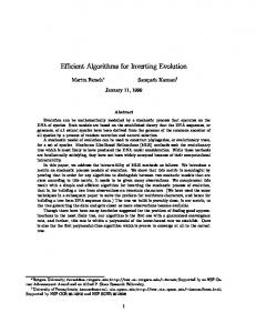


![[PDF] Storing Energy: with Special Reference to Renewable Energy ...](https://m.moam.info/img/260x300/pdf-storing-energy-with-special-reference-to-renew_6477e6d3097c4744708c3ac3.jpg)


