path tracking controllers during manoeuvring over slippery and rough terrains. ... The trials were carried out in an agricultural machinery, skid steer loader Cat R.
2016 IEEE/RSJ International Conference on Intelligent Robots and Systems (IROS) Daejeon Convention Center October 9-14, 2016, Daejeon, Korea
Probabilistic Approaches for Self-tuning Path Tracking Controllers using Prior Knowledge of the Terrain Alvaro Javier Prado1 , Fernando Auat Cheein1 and Miguel Torres-Torriti2 Abstract— Nowadays, agricultural and mining industry applications require saving energy in mobile robotic tasks. This critical issue encouraged us to enhance the performance of path tracking controllers during manoeuvring over slippery and rough terrains. In this scenario, we propose probabilistic approaches under machine learning schemes in order to optimally self-tune the controller. The approaches are real time implemented and tested in a mining machinery skid steer R 262C under gravel and muddy terrains (and their loader Cat transitions). Finally, experimental results presented in this work show that the performance of the controller enhances up to 20% (average) without compromising saturations in the actuators.
I. INTRODUCTION Agriculture and mining robots generally perform cycling precision tasks in controlled environments. For instance: seeding, crop sensing, weeding and other followed-up operations [1], [2], following a previous planned path, whereas other robots (e.g., robots devoted to mining processes) execute functions in extreme conditions of rough, slippery, uneven, or even more steep terrains [3], [4], [19] among others. The latter constrains may be impossible or exceedingly costly to be conditioned for a safe and robust path planner [5]. Thus, taking advantage that robots performs repetitively tasks, one can make the robot learn some characteristics in order to refine the performance of path tracking controllers based on some previous knowledge of the environment [6]. Although path tracking controllers with constant parameters should be designed for suitable responses to disturbances, some of these controllers would make a great effort over the control commands to achieve an initial defined performance. Actually, the transient response would make the robot to waste considerable amount of valuable energy [7]. On the other hand, a wide gamma of path tracking controllers with adaptive parameters have been proposed in the literature. For instance, a path tracking controller with adjustable parameters considering non-linear saturations in the actuators and the dynamic model is presented in [8]. A similar approach for adaptable self-tuning gains based on the kinematic model of the robot and Llyapunov-stability analysis is shown in [9]. Furthermore, model-free controllers designed to follow planned paths based on adaptivity techniques, such as fuzzy systems, neural networks and genetic This work is founded by the CONICYT-PCHA/Doctorado Nacional/2015-21151095, FONDECYT Grant 1140575, Basal Grant FB0008, DGIIP-UTFSM Chile and Pontificia Universidad Cat´olica de Chile, Chile. 1 Department of Electronic Engineering, Universidad T´ ecnica Federico Santa Maria, Valparaiso, Chile 2 School of Electrical Engineering, Pontificia Universidad Cat´ olica de Chile, Chile
978-1-5090-3762-9/16/$31.00 ©2016 IEEE
algorithms respectively, are shown in [10], [11], [12]. As can be seen, researchers have addressed efforts to enhance the performance of path tracking controllers considering the robot’s model or the path, but few have dealt with the characteristics previously known of the ground. In this work, a pair of probabilistic approaches to find optimal set of gains for path tracking controllers are presented and tested in the field. The methodologies are based on machine learning techniques taking advantage of the prior knowledge of the terrain. The optimal set of gains are found such that minimize the path tracking error, the effort of the controller and the effects of the slippage when a robotic vehicle navigates over two type of terrains (suggested in [13]): gravel and mud. The methodologies were evaluated considering a square-shaped path (suggested in [14]) and tested in a controller previously presented in [1]. The performance of the controller was evaluated with the metrics stated in [15]: the total error cost, the total effort and the slippage cost. The two methodologies are base on finding optimal set of gains from a training set previously generated with a Monte Carlo approach. The first methodology assumes that the training set is a mix of Gaussian distributions that must be clustered to find the best estimation, whereas the second approach considers means of Gaussian distributions shifting in mobile-windows in the direction of the gradient ascent. The trials were carried out in an agricultural machinery, skid R 262C (automated for this work). steer loader Cat This paper is organized as follows: Section II describes a brief overview of the hardware where the trials were carried out, the path tracking controller formulation, the metrics to measure the performance of the controller and the method to generate the training set. Section III presents the methodologies proposed in this work. Section IV shows the previous preparation to the experimentations and the results obtained in the implementation of the methodologies. Section V shows the conclusion of this work. II. SYSTEM OVERVIEW The vehicle used in this brief is a compact industrial maR 262C, generally employed chinery –skid steer loader Cat for mining purposes. This robotic vehicle was automated at the School of Electrical Engineering, Pontificia Universidad Catolica de Chile, Santiago de Chile. The system includes an electronic board (Master Board MK1) to interface the electronic components with the vehicle and an on-board computer used to implement our proposal. In addition, the algorithms are implemented in C/C++, Python 2.7 and Matlab. The vehicle is equipped with a differential GPS antenna
3095
as shown in Eq. 3. Ω Cx,y = •
ρ 2
P#Ω
t=0 (xt
− xref,t )2 + (yt − yref,t )2
(3)
The Total effort is related to the amount of wasted kinetic energy while the robotic vehicle tracks the predefined path, as shown in Eq. 4. Ω CV,ω =
γ 2
P#Ω
t=0
Vt2 + ωt2
(4)
Fig. 1: Platform used to carry out the trials.
(from Swift Navigation), a high precision inertial module unit (IMU NAV2000, from Vector Navigation Technologies) and vehicle’s inner encoders on the front wheels. A. Robot Model and Path Tracking Controller The motion model considered for this robotic vehicle is the uncycle model. The governing equations are defined as follows: xt+1 xt Vt cos(θt ) yt+1 = yt + ∆t Vt sin(θt ) (1) θt+1 θt ωt where Vt and ωt are the control commands: linear speed and angular velocity respectively. [xt yt θt ]T is the pose of the robot at instant of time t with respect to a global reference frame previously established. For this work, the sampling time of the system is set to ∆t = 0.1 seconds. Our approaches were implemented in the controller previously published by Auat & Scaglia [1]. However, the methodology presented herein can be extended to other controllers. The controller used in this brief is focused on an algebraic approach with three parameters or set of gains K = [kx ky kθ ]T . Equation 2 shows the governing expressions with its corresponding set of gains, and also the boundary constrains for ensuring stability. 1 Vt = � ∆t (∆x cos θez,t + ∆y sin � θez,t ) θez,t+1 −kθ (θez,t −θt )−θt ωt = ∆t (2) ∆x = xref,t+1 − kx (xref,t − xt ) − xt ∆y = yref,t+1 − ky (yref,t − yt ) − yt 0 < kx , ky , kθ < 1 where [xref,t yref,t ]T represents the desired position, and θez is the orientation angle between the reference trajectory and the current position of the robotic vehicle based on the controller formulation. More details about the controller and its implementation can be found in [1]. B. Performance Costs In this work, we used the following metrics to quantify the performance of the path tracking controller under changes in the terrain characteristics, following the guidelines shown in [15]. Briefly, • The Total error cost is the sum of the errors between the position of the vehicle and the trajectory to be tracked,
In this brief, we considered an additional metric: the slippage cost, as shown in Eq. 5. This consideration takes into account the coefficient-slippage (λ) between the robotic vehicle’s wheels and the different type of terrains where the vehicle travels. P#Ω tR , Vt 6= 0 (5) CλΩ = σ2 t=0 λ2t , where λt = Vt −ω Vt where #Ω is the total number of points used to generate the reference trajectory Ω. In addition, the friction coefficient-slippage (λ) can be calculated, considering kinematic conditions in the robotic vehicle, as the difference between the longitudinal velocity (Vt ) and the traction velocity (ωt R, where R is the radius of the vehicle’s wheel) normalized by its longitudinal velocity. Note that λ can only be calculated when the longitudinal velocity is different from zero, thus the proposed slippage cost in Eq. 5 is calculated considering this constrain [18]. Equation 5 shows a simple formulation of slippage considering the two independent variables Vt and ωt . Additionally, ρ, γ and σ are constant parameter used to give priority to the cost functions. C. Monte Carlo seeds Generation The controller parameters K = [kx , ky , kθ ]T can vary according to a required performance. In this work, the set of gains K are selected pseudo-randomly as a function of the system response, the controller formulation and the metrics previously stated in Section II-B. This procedure is depicted in Algorithm 1. Lines of code (1)-(4) show the initial conditions to generate the Monte Carlo seeds. Note that in line of code (2) each parameter kx , ky , kθ is assumed to follow a Gaussian distribution in the domain kx,y,θ ∈ [0, 1]. The for-loop –lines of code (5)-(23)– generate points #Ω while the robot is moving, whereas the inner for-loop –lines of code (6)-(22) – is the core of the algorithm. As can be seen in lines of code (10)-(21), the Monte Carlo method selects the set of gains Kf inal providing a lower error cost, reduction of the total effort and a minor slippage cost per iteration. This method allows us to generate the set of gains that do not exceed saturation constrains –see line of code (10). In this work, we considered N = 1000 random set of gains K, and the Monte Carlo approach provided around 800 seeds along the path. The points were generated at sample time ∆t = 0.1 seconds.
3096
Algorithm 1 Generation of Monte Carlo seeds to find K
Algorithm 2 First Approach: Gaussian Mixture Model
1: Let N be the maximum number of Monte Carlo seeds. 2: Let K 0 = [kx ky kθ ]T a random set of gains following a Gaussian distribution in the domain K ∈ [0, 1]. 0 , C 0 0 3: Let Cx,y = Cx,y V,ω = CV,ω and Cλ = Cλ be the initial costs stated in Section II-B obtained with the set of gains in code line (2). These costs are obtained as soon as the vehicle starts to move. 0 + C0 0 0 4: Calculate CT0 ot = Cx,y V,ω + Cλ with K . 5: for t = 1 to #Ω do 6: for j = 1 to N/#Ω do 7: Generate random K j with Gaussian distribution in its domain K ∈ [0, 1]. 8: Calculate the control commands [Vt , ωt ] when the vehicle has started or stopped considering the controller in Section II-A. j j , CV,ω 9: Calculate the costs Cx,y and Cλj following Section II-B. j j−1 j j−1 10: if Cx,y < Cx,y , CV,ω < CV,ω , Cλj < Cλj−1 , Vt < V max and ωt < ω max then j j , CV,ω 11: Save Cx,y , Cλj j 12: Knew = K j 13: else j = K j−1 14: Knew 15: end if j j j 16: Calculate the total cost CTj ot = Cx,y + CV,ω + Cλj with Knew . j j−1 17: if CT ot < CT ot then j 18: Kfj inal = Knew 19: else 20: Continue with the procedure. 21: end if 22: end for 23: end for
1: 2: 3: 4: 5: 6: 7: 8:
9: 10: 11: 12: 13: 14: 15: 16: 17: 18: 19: 20: 21: 22: 23: 24:
Let c be the number of centroids of the clusters. Let m be the number of samples –Monte Carlo seeds. n . Initialize Σ ∈ S++ n . Initialize a matrix of weights δ ∈ S++ Let αj ∈ Rn be a vector of independent and identically distributed latent variables, where j = 1, .., c for j = 1 to c do for i = 1 to m do Calculate the weights δji as the quotient between the Gaussian i distribution: N P(K , µj , Σj ) and the sum of weighted Gaussian distributions cj=1 αj N (K i , µj , Σj ). end for end for for j = 1 to c do for i = 1 to m do Calculate the latent vector αj as the weights δji normalized for m. Calculate the estimation of the set of gains µj weighting them with δji . Update the covariance matrix Σj with Pm (i) (i) T − µj )(K (i) − µj ) . i=1 δj (K end for end for (i) if log l(Kj , α, Σ, µ) converges ∀i = 1, ..., m and j = 1, ..., c then ˆ j = µj , ∀j = 1, ..., c. Assign the final calculated means as: K Save the covariance matrix Σj , ∀j = 1, ..., c. Break. else Continue with the process. end if
III. CLUSTERING STRATEGIES In this work, we propose two methodologies for selecting the appropriate set of gains based on clustering the training set obtained from the Monte Carlo seeds generation in Section II-C. It is worth mentioning that the approaches presented herein can be applied regardless of the robot model formulation. A. Gaussian Mixture Model: GMM This first method is focused on a maximum a posteriori approach in order to group the training set based on finding ˆ and its covariance matrix Σ associated the best set of gains K to the propagation error [16]. The optimization problem can be depicted as shown in Eq. 6. ) ( m Y (i) ˆ = argmax p(K |α, Σ, µ) (6) log K K∈Rn
The maximization problem formulated in Eq. 6 is solved in lines of code (11)-(17) updating the mean µ and the covariance matrix Σ for every cluster. The algorithm stops when the log-likelihood associated to the argument of the Eq. 6 converges, see code lines (18)-(24). The estimated set of gains obtained in the Algorithm 2 represents the centroids of every cluster, then all the set of gains in the training set is labelled to every cluster according to a function of membership fm (see Eq. 7) where the selection criteria consists of comparing the distances between the set of gains of the training set and the estimated set of gains of every cluster. In this work, the cluster such that the minor distance between two set of gains is measured will correspond to the selected cluster.
fm =
i=1
where K (i) is the ith set of gains in the training data, assuming this set of gains following a Gaussian distribution with mean µ and covariance matrix Σ; m is the number of samples, n represents the dimension of the Monte Carlo seeds and α is a latent membership variable associated to ˆ every distribution p(K i |α, Σ, µ). The procedure to find K and Σ is shown in Algorithm 2. In lines of code (1)-(5), the parameters of the algorithm are initialized. Among these parameters, the number of clusters to group the training set c is a designer criterion. Lines of code (6)-(10) show the procedure to determinate a matrix of weights δ used to modify the estimation of the set of gains at every iteration of the algorithm.
(i) K (i) → Kj
0
ˆ j ) < d(K (i) , K ˆ l) , if d(K (i) , K ∀j, l = 1, .., c and i = 1..., m with j 6= l , otherwise
(7)
where m represents the length of the training data, c is the amount of pre-defined clusters and Kji is the set of gains of the training data labelled to the corresponding cluster j, d(·, ·) is the metric stated to define the clusters; in our case the Malanhobis distance. The membership function describes a case where a certain set of gains may not belong to any cluster, this is due to the fact that some set of gains are outliers of the model. B. Mobil-Window Clustering: MWC This approach assumes every point in the training set follows a Gaussian distribution p(K) ([17]), similar to the
3097
first approach as can be seen in Eq. 8 . However, this method can use other distributions to obtain the best estimations for some given application. In addition, we assumed a mobilwindow around every point in the training set to be shifted in the direction of the gradient ascent where the density of points is higher, see Eq. 9. The gradient of the distribution defines the mean shift vector m(K) which points to the ˆ within a certain cluster that contains the best estimation K most probable points of the training set. This estimation is calculated as can be seen in Eq. 10. f (K) =
m � X �T � � −1 1 K − µi K K − µi Σ n −1 m|Σ | i=1
µi = µi + νm(K) � � �T � m K − µi Σ−1 K − µi i=1 Ki K � � − K m(K) = P m i −1 (K − µi )T i=1 K (K − µ ) Σ
(8) (9)
P
(10)
where K represents the distribution that every point in the training set follows. For this approach, a Gaussian distribution. The speed of convergence is defined by ν. The procedure can be described as follows: the initialization is as the previous algorithm. Additionally, it considers a process covariance matrix Q. Every point in the training set is evaluated through a small window with a bandwidth defined by the difference between the maximum and minimum set of gains –lines of code (4)-(5). In lines of code (6)-(13), for every point in the data set the window shifts whereas the vector m(K) is calculated. The estimation µ is updated with the vector m(k) until µ converges. The covariance matrix Σ is updated similarly as the estimation of K. However, this matrix is weighted with the gradient of the distribution f (K). The resulting estimation is compared with the previous ˆ to check if it is different from the previous estimations of K ones. Finally the estimation µ is saved to be used in the clustering of the training set, see lines of code (14)-(20). ˆ are used to cluster the At this point, the estimations K training set according to the membership function stated in Eq. 7. IV. EXPERIMENTAL RESULTS To validate our hypothesis, we tested our probabilistic self-tuning approaches in two different terrains: muddy and gravel. First, we obtained the training set in the field according to the algorithm presented in Section II-C and then clustered in order to obtain a proper set of gains according to the algorithms presented in Section III-A and III-B. The resulting set of gains are used to implement the controller with the same initial conditions and then finally we evaluated the performance of the controller in terms of the metrics stated in Section II-B. A. Experimental preparation The squared shaped path implemented in this work contains #Ω = 300 waypoints separated uniformly with a distance of 0.1 m. The initial pose of the robotic vehicle is aligned to the initial point of the path. To evaluate the algorithms presented in Section III-A and III-B, we
Algorithm 3 Second Approach: Mobil-Window Clustering 1: 2: 3: 4: 5: 6: 7: 8: 9: 10: 11: 12: 13: 14: 15: 16: 17: 18: 19: 20: 21:
n . Initialize a matrix Q ∈ S++ Select an aleatory point in the training set as starting K. Let υ a bandwidth factor of a certain window W Select the minimum Kmin an maximum Kmax value of the training set. Calculate the bandwidth of the window: W = υ [Kmax − Kmin ]. for i = 1 to m do repeat Calculate µi and m(K) with Eq. 9 and Eq. 10 respectively, bounded with the bandwidth P W. (i) . Calculate K with K = m i=1 m(K)K n Calculate Φ ∈ S++ with Φ = ∇f (K). Calculate the covariance matrix Σi+1 = ΦΣi Φ + Q. Move the window W one step ahead. until d(µi , old µ) < λ ˆ ← µi . Assign K ˆ old K) ˆ < � then if d(K, Continue with the process else ˆ Save K, Save Σ. end if end for
considered a strategic workspace where the corner of the squared path matches with the change of terrain required in this work. Previous the implementation of the path tracking controller, the optimal set of gains are obtained considering the following: (i) we first generated the training set according to the stated in Section II-C using pseudo-random set of gains max min ] = [0.1, 0.9]. This algorithm , Kx,y,θ bounded by [Kx,y,θ delivered around 800 Monte Carlo seeds per training set, two training sets one per type of terrain. (ii) Each training set is clustered with the two approaches mentioned in Section III-A and Section III-B. For the first approach (GMM) four clusters are considered, whereas in the second approach (MWC) the amount is automatically calculated; and (iii), for visualization purposes, we show a representative amount of Monte Carlo seeds together with the distribution of the groups and the clusters of the training set, for the two approaches and the two experimental cases –see Figs. 2a to 3d. For the first case, the two approaches (GMM and MWC) are implemented to cluster the training set to obtain the optimal set of gains – see Figs. 2a-2d. The groups of the training set formed for the first approach (GMM) can be seen in Fig. 2a, and the clustering of the training set is depicted in Fig. 2b, whereas in the second approach (MWC) the groups are formed as can be can be seen in Fig. 2c and the clusters in Fig. 2d. Note that Fig. 2a and Fig. 2c show the distribution of the training set considering the plane kx − ky, respectively. In Fig. 2a, the magenta surface represents the higher probability ˆ and the green surface the lower to find the optimal gain kθ one. Moreover, the level curves showed in the plane ky − kθ and kx − kθ show the distribution of probability to find the ˆ and ky ˆ respectively. These set of gains can best gains kx bee seen in the gray plane of the Fig. 2a, where the whiter area shows the higher density of points. Once the optimal set of gains are obtained for every case, the clusters are formed according to the membership
3098
(a)
(a)
(b)
(b)
(c)
(c)
(d)
(d)
Fig. 2: Groups and clusters of training set obtained in trial over muddy terrain: Fig. 2a shows the projection over the ˆ Fig. 2b shows a superior plane kx − ky of the estimation K, sight of the distributions per group, Fig. 2c shows the level curves of the groups in every plane, Fig. 2d shows the clusters in every plane.
Fig. 3: Groups and clusters of training set obtained in trial over gravel terrain: Fig. 3a shows the projection over the ˆ Fig. 3b shows a superior plane kx − ky of the estimation K, sight of the distributions per group, Fig. 3c shows the level curves of the groups in every plane, Fig. 3d shows the clusters in every plane.
B. Field results function stated in Eq. 7. For the first transition of terrain (asphalt to gravel), Fig. 2b and Fig. 2d show the training set clustered using the two proposed approaches (GMM and MWC, respectively). The yellow, magenta and green points corresponds to the three clusters obtained in the training set, while the blue points do not correspond to any cluster. Additionally, Figure 2b shows the Gaussian distributions of each cluster around the training set, and clearly the density of points changes in order to reach the best performance due to transitions in the surfaces of terrain. Finally, Figures 3a3d show similar results considering the second experimental case; changing from asphalt to muddy terrain.
The optimal set of gains obtained in the previous section are used to set the parameters of the proposed controller Auat & Scaglia [1]. The trials were carried out remaining the square-shaped path and the initial conditions as in the previous section. Additionally, we considered the changes in the terrain previously described in Section IV-A, the system responses for the first experimental case –muddy ground– and second case –gravel terrain– can be seen in Fig. 4a and Fig. 4b respectively. The solid black line represents the reference path and the other three dashed lines are the tracked path considering a constant setting of K (blue dashed line) and the set of gains obtained in the two approaches (GMM
3099
(a)
training set is a mix of Gaussian distributions, whereas the second one (MWC) finds the optimal set of gains shifting means of Gaussian distributions in a pre-defined mobilewindow. Experimental results show encouraging results in terms of tracking error, total effort of actuators and low slippage cost; 20% average. This means the performance of the controller improved and lower energy is wasted through difficult conditions of terrain.
(b)
Fig. 4: Experimental results: Fig. 4a shows the transient response in muddy terrain with the two approaches and constant set of gains, whereas Fig. 4b shows the transient response under gravel terrain.
(a)
(b)
(c)
(d)
(e)
(f)
Fig. 5: Costs obtained in the experimentations: Figs. 5a, 5c and 5e show the costs obtained when the robot moves in muddy terrain, considering the constant set of gains and the two approaches, whereas Figs. 5b, 5d and 5f show the costs obtained for the second case.
and MWC) (red and magenta dashed lines). The results obtained in Fig.4a and 4b show similar responses for the two approaches, however the results obtained by the two methodologies are better than those obtained maintaining a constant set of gains K. Figures 5a, 5c and 5e show the accumulative tracking error, the accumulative slippage cost and total cost respectively, for the first case where the vehicle navigates through muddy terrain, whereas Figures 5b, 5d and 5f show the performance of the controller for the second case where the vehicle tracks the path through gravel terrain. V. CONCLUSIONS The methodologies are based on probabilistic approaches using a prior knowledge of the set of gains (training set) in order to cluster them and then estimate the optimal set of gains. The first approach (GMM) considers that the
R EFERENCES [1] F. Auat Cheein, G. Scaglia. Trajectory Tracking Controller Design for Unmanned Vehicles: A New Methodology, Journal of Field Robotics, in press, 2014, DOI: 10.1002/rob.21492. [2] R. Eaton. Precision Guidance of Agricultural Tractors for Autonomous Farming, Montreal, Que, pp. 1-8, 2008. [3] M. Burke. Path-following control of a velocity constrained tracked vehicle incorporating adaptive slip estimation, Saint Paul, MN, pp. 97-102, 2012. [4] A. K. Singh and D. Ghose and K. M. Krishna. Optimum steering input determination and path-tracking of all-wheel steer vehicles on uneven terrains based on constrained optimization, Montreal, QC, pp. 3611-3616, 2012. [5] Yi Guo and L. E. Parker and D. Jung and Zhaoyang Dong. Performance-based rough terrain navigation for nonholonomic mobile robots, vol. 3, pp. 2811-2816, 2003. [6] M. Reinstein and V. Kubelka and K. Zimmermann. Terrain adaptive odometry for mobile skid-steer robots, Karlsruhe, pp. 4706-4711, 2013. [7] M. Ashoorirad and R. Barzamini and A. Afshar and J. Jouzdani. Model Reference Adaptive Path Following for Wheeled Mobile Robots, Shandong, pp. 289-294, 2006. [8] M. D. Adams. Adaptive motor control to aid mobile robot trajectory execution in the presence of changing system parameters, IEEE Transactions on Robotics and Automation, vol. 14, pp. 894-901, 1998. [9] J. Seung. Adaptive tracking and obstacle avoidance for a class of mobile robots in the presence of unknown skidding and slipping, IET Control Theory & Applications, vol. 5, pp. 1597-1608, 2011. [10] P. Saeedi and P. Lawrence and D. Lowe and P. Jacobsen and D. Kusalovic and K. Ardron and P. Sorensen. An autonomous excavator with vision-based track-slippage control, IEEE Transactions on Control Systems Technology, vol. 13, pp. 67-84, 2005. [11] T. T. Hoang and D. T. Hiep and B. G. Duong and T. Q. Vinh, Trajectory tracking control of the nonholonomic mobile robot using torque method and neural network, Melbourne, VIC, pp. 1898-1803, 2013. [12] J. Guo and P. Hu and L. Li and R. Design of Automatic Steering Controller for Trajectory Tracking of Unmanned Vehicles Using Genetic Algorithms, IEEE Transactions on Vehicular Technology, vol. 61, pp. 2913-2924, 2012. [13] T. Luettel and M. Himmelsbach and H. J. Wuensche. Autonomous Ground Vehicles #x2014;Concepts and a Path to the Future, Proceedings of the IEEE, vol. 100, pp. 1831-1839, 2012. [14] S. Roth, P. Batavia. Evaluating path tracker performance for outdoor mobile robots. In http:www.ri.cmu.edupublication view.html?pub id=3908, retrieved September, 2014. [15] S. Blaic. A novel trajectory-tracking control law for wheeled mobile robots, Robotics and Autonomous Systems, Vol. 59(11), pp. 10011007, 2011. [16] Basri and Indrabayu and A. Achmad, Gaussian Mixture Models optimization for counting the numbers of vehicle by adjusting the Region of Interest under heavy traffic condition, Surabaya, pp. 245250, 2015. [17] M. A. Carreira-Perpinan. Gaussian Mean-Shift Is an EM Algorithm, IEEE Transactions on Pattern Analysis and Machine Intelligence, vol. 29, pp. 767-776, 2007. [18] R. Jazar. Vehicle Dynamics Theory and Applications, Springer, NY USA, 2008. [19] Fernando A. Auat Cheein, Gustavo Scaglia, Miguel Torres-Torriti, Jos Guivant, Alvaro Javier Prado, Jaume Arn, Alexandre Escol, and Joan R. Rosell-Polo. Algebraic path tracking to aid the manual harvesting of olives using an automated service unit. Biosystems Engineering, 142:117 – 132, 2016.
3100