Probabilistic inference as a model of planned ... - Semantic Scholar

Probabilistic inference as a model of planned behavior Marc Toussaint The problem of planning and goal-directed behavior has been addressed in computer science for many years, typically based on classical concepts like Bellman’s optimality principle, dynamic programming, or Reinforcement Learning methods – but is this the only way to address the problem? Recently there is growing interest in using probabilistic inference methods for decision making and planning. Promising about such approaches is that they naturally extend to distributed state representations and efficiently cope with uncertainty. In sensor processing, inference methods typically compute a posterior over state conditioned on observations – applied in the context of action selection they compute a posterior over actions conditioned on goals. In this paper we will first introduce the idea of using inference for reasoning about actions on an intuitive level, drawing connections to the idea of internal simulation. We then survey previous and own work using the new approach to address (partially observable) Markov Decision Processes and stochastic optimal control problems.

1

Probabilistic inference and internal simulation

Models of intelligent behavior organization can be roughly distinguished as model-based or model-free. In a model-free approach the sensorial input (or the state1 ) is directly mapped to actions and motor signals without the need to anticipate what the outcome of these actions might be. In the context of cognitive science one would describe such an action selection system as reactive or habit-based [2]. An agent that follows a model-free approach can learn to behave optimally by associating a certain value to states and actions – which is the core idea of classical Reinforcement Learning (RL) methods [30] – but it will not be able to predict or anticipate where these actions lead. In fact, there is no role for anticipation (or general knowledge) except for the prediction of the expected future reward depending on the state. The mapping from state to action is one-way – since the agent cannot anticipate, the sensor-motor loop can only be closed by explicit (“overt”) interaction with the external world. Model-free behavior organization is without doubt a fundamental aspect of human and animal behavior (reflexes, habits, motor skills), but it does not account for planned and anticipatory behavior. In contrast, in a model-based approach the ability to predict (even if with uncertainty) is essential. One assumes that some model of the environment is available or has been learnt from experience. Given such a model one can in some sense close the loop internally, i.e., predict the change of stimuli and world state depending on (“covert”) actions and thereby induce an internal simulation of action sequences and effects. Clearly, internal simulation provides a very intuitive idea of how a learnt model of the world can be used for decision-making and goaldirected, prospective behavior. However, from a theoretical and computer scientist point of view we would like to have a more rigorous framework and efficient computational model of such processes. In this paper we discuss a new computational method for planning and control based on probabilistic inference, which can 1 We

will more precisely discuss partial observability later.

be thought of as a theoretically grounded formalization of the idea of internal simulation. We will show later to what degree the inference approach and classical reinforcement learning and control methods are equivalent. Let us first try to pinpoint the core ideas of the inference approach in a minimalistic but formal setting. Probabilistic inference is a method to infer estimates of unobserved variables. For instance, let X and Y be two random variables that are coupled by some conditional probability P (Y |X) (e.g., a measurement device). Graphically this can be expressed as X

Y

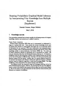
Assume we observe only Y (a measurement) and want to estimate X (the true state). When we have a prior P (X) over X we can compute a posterior distribution P (X|Y ) ∝ P (Y |X)P (X) using Bayes rule. This approach has been pervasive and successful in many applications for decades: In Kalman filters (X is a true trajectory, Y measurements of the trajectory), in speech recognition (X is a sequence of phonemes, Y measured auditory features), in image processing (X are true pixel colors, Y a noisy image), etc. As a result, probabilistic inference methods have for decades been used in the context of sensor processing: given measurements, the true state of an unobserved variable is estimated. However, more generally inference methods can be understood as a computational paradigm that relaxes to a coherent estimate of coupled variables2 . This principle can not only be applied to sensor processing but also to the estimation of actions and decisions that are coherent with constraints and goals: Assume we have three random variables X, Y , and Z coupled as X

Y

Z

Assume we know X (“where we are”) and we know Z (“where we want to be”) – we can use inference methods to estimate Y , 2 To stay formally precise, we could identify the notion of “coherence” with the marginal consistency property in factor graphs.

i.e., estimate the intermediate step that is “coherent” with observed information (X) and the goal (Z). This, in a nutshell, is the idea of using inference to reason about actions. The beauty of the idea is that the network of involved coupled variables can include a multitude of variables, some of which might represent known features of the current state, some of which might represent constraints, goals, or motivations that lie in the future, and some of which might represent future actions, motor signals, sensor signals or any other kind of information. The variables can be discrete, continuous or mixed, they can represent hierarchies and abstractions. The decision or planning process now means to clamp (condition) some of these variables to desired values (goals), others to known context or sensor information, and then to use a computational machinery that yields coherent estimates of variables (in particular actions) across the network. The next section will express this more formally in the framework of graphical models.

2

Networks of actions, goals and sensor variables

A convenient – but surely not the only possible – mathematical framework to formalize these ideas are so-called (dynamic) Bayesian networks [17, 22]. In this framework we think of the state at a certain time as being described by a number of random variables. When we discretize time uniformly (which we do here for simplicity) we have these random variables in each time slice. A dynamic Bayesian network (DBN) describes the collection of all random variables and their coupling in a temporal process. In a more intuitive sense, the DBN represents our future spread out in front of us. All these variables are coupled somehow. Apart from a prior that we might have, all these variables are yet undetermined since they represent events or features of the future which are yet not observable. In this framework goals correspond to “mental observations” of future events – they correspond to conditioning some random variables in the DBN (clamping them to a fixed value). To give an example, when we walk past an advertisement for an ice cream, this might inevitably induce the “mental observation” of ourselves eating the ice cream somewhere in the future3 , that is, the conditioning of some variables in our DBN model of the future. In Graphical Models [17], inference is the process of computing a posterior marginal over all variables given that some variables are observed and we know how the variables are coupled. Let us describe in some more detail what inference algorithms actually do (following the framework of factor graphs [19]). Formally, they assume that a so-called joint probability distribution Y Y P (X1 , .., Xn ) = φi (Xi ) ψij (Xi , Xj ) i

·

Y

(ij)

χijk (Xi , Xj , Xk ) · · ·

(1)

(ijk) 3 Note the use of “somewhere” – the undeterminedness of when we eat the ice cream (and receive the reward) is non-trivial to handle properly. The mixture of DBNs in section 3.2 will be our solution to this “somewhere”.

defines a scalar function over a tuple (X1 , .., Xn ) of random variables. As expressed in the above equation, one assumes that this function can be factored in variable-wise potentials φ, pairwise couplings ψ, triple-wise couplings χ, etc. Generally, one writes Y P (X1:n ) = ψC (XC ) (2) C

in terms of cliques C which are subsets of coupled variables. Observations correspond to potentials φi which are zero except for the value of Xi which is actually observed. Inference computes the marginal beliefs b(Xi ) for a variable Xi , i.e., computes the distribution of Xi when all global information, couplings, and observations are taken into account. Inference methods like belief propagation can be interpreted as a computational scheme that tries to achieve consistence between coupled marginal beliefs, that is, when XC and XD represent two cliques that share a variable posterior beliefs should coP Xi , then their marginal P incide, XC \Xi b(XC ) = XD \Xi b(XD ) (see [32] for a brief technical introduction to factor graphs and belief propagation). This corresponds closely to methods in statistical physics that try to estimate the state distribution of a large number of particles when they are locally coupled but also fulfill constraints (observations), e.g., at boundaries. What does this imply for our ice cream example? When we assume that there is an inference machinery permanently active on our DBN, then the ice cream advertisement conditions a variable describing ourselves eating the ice cream, the inference machinery immediately infers what this implies for all the other variables in the network – in particular the future that lies between now and the ice cream. In some sense the inference machinery completes the picture of our future and lets us imagine also all the intermediate steps toward the ice cream. We haven’t explicitly discussed actions yet. Interestingly, in this framework there is hardly need to distinguish between action or motor variables and state features or sensor variables. The DBNs may include all kinds of variables equally, sensor variables, motor variables, abstractions, reward variables, continuous and discrete variables; whatever representations are available. The inference machinery only computes what the conditioning of one variable implies on the others, independent of whether they might correspond to actions or perceptions. When our DBN includes motor and action variables, then the conditioning of some future variable will imply an effect on the immediate motor or action variable. If we make a last assumption that a non-uniform posterior on an action variable inevitably leads to the overt execution of the action, then we closed the loop: We see the ice cream, the mental observation is induced, the inference machinery spreads its messages through all other variables, the posterior of some action or motor variables becomes non-uniform, we execute the action. The ice cream example gives a plausible idea of the working of probabilistic inference in the context of goal-directed behavior, but we should complement this intuitive example with some critical remarks: First of all, the above view is suggestive in that this is how the brain might work – but do we have evidence for this? Answers to this can be given on different levels. On a purely information processing level, several authors proposed that certain functions of neural substrates could be abstracted in terms of Bayesian information processing and inference [10, 24].

On a neuroscientific level, Johnson and Redish [16] were able to record neural activation patterns in rats during path planning that are remarkably similar to a spatial forward simulation. On a cognitive level, Botvinick and An [2] argues rather closely along the above lines of thought; Hesslow [13] and Grush [11] generally discuss the role of internal simulation and imagery and propose, for instance, Kalman filtering as a computational model of internal simulation. These studies encourage our view that probability inference might serve as an interesting model of neural functions – but clearly this hypothesis should be considered tentative before we have more evidence in this direction. As a second remark, the picture above suggests that we are done after a single inference pass. However, when establishing relations to computing optimal policies in Markov Decision Processes (MDPs) (next section) we will find that one needs an additional (Expectation Maximization, EM) loop on top of the inference machinery. This is inevitable since the optimal action now depends on the actions taken in the future. So, a model of the future from which we can infer the optimal immediate action needs to “use” the optimal policy in the future – this recursive loop is resolved with an EM algorithm. Nevertheless, we belief that the general picture we sketched in this section is useful (1) as an inspiration for new approaches to behavior organization and (2) as an intuitive grounding to better understand the concrete computational methods we have developed in recent years, which proved very efficient in concrete applications and which we survey in the following section.

3

stochastic optimal control [21]. Cano et al. [5] use Monte Carlo methods for computing optimal policies in continuous state influence diagrams. There are some crucial differences between the framework of influence diagrams and temporal process models such as MDPs or stochastic optimal control; see [3, section 4.3] for an excellent discussion. One point is that influence diagrams typically describe finite worlds whereas MDPs describe infinite processes. While inference methods in influence diagrams rely on recursing backward starting from the last decision, there is no “last decision” in an infinite-horizon MDP. Further, in stationary MDPs the optimal policy is known to be stationary, i.e., independent of time and needs to be optimized globally. Instead, in influence diagrams each decision can be treated separately (in backward order). Indeed, in textbooks on influence diagrams [18] the infinite-horizon or stationary sequential decision problem is addressed based on the Bellman optimality equation and recursive value function computation. To my knowledge, inference methods for solving infinite-horizon or stationary scenarios have not been developed in the context of influence diagrams. Beyond influence diagrams, there are a series of papers that investigate inference methods in MDPs. Attias [1] assumed that instead of arbitrary rewards at every time slice we have one goal state g at the final time (which can easily be generalized to several goal states), and a finite horizon T is prefixed. Additional sequential dependencies between actions are also assumed. Given this model, Attias computes the MAP (maximum aposteriori probability) action sequence conditioned on reaching the goal,

Concrete Methods

∗ α0:T -1 = argmax P (a0:T -1 | xT = g) .

(3)

a0:T -1

In this section we survey a series of explicit realizations of the above concept. Instead of going into all technical details in each case we refer to the technical publications. Our aim is to show that the concept can be applied consistently in a variety of cases and is not limited to, say, only MDPs. We will discuss • previous work, in particular on influence diagrams, • a new method to compute optimal policies in MDPs, • an extension to hierarchical POMDPs, • a new method to approximately solve stochastic optimal control problems, • and briefly some other extensions.

3.1

Previous work & Influence Diagrams

The idea of using inference methods for reasoning about decisions has a long history. The earliest work on this we are aware of was done in the context of so-called influence diagrams [14]. A key to the application of inference methods was to replace the utility functions (scalar functions that measure cost or reward) by a random variable which represents a “success event” such that success probability is proportional to the total utility. This idea is presented in [7, 25, 28]. The early approaches to use inference made very strong assumptions (one utility variable, regularity, no-forgetting) which leads to inefficient algorithms (the no-forgetting assumption immediately lets the clique size explode). Later work remedied some of these inefficiencies by considering multiple utility variables and better exploiting the problem structure [15, 41]. Kjaerulff and Madsen [18] present a modern text book on influence diagrams including interesting work on solving continuous state problems similar to LQG

The paper was very inspiring for the subsequent work, although the method does not exactly solve the typical MDP problem in the sense of computing a policy that maximizes future expected return. Raiko and Tornio [27] introduced the same idea independently in the context of continuous state stochastic control and called this optimistic inference control. Verma and Rao [38] used inference to compute plans (considering the maximal probable explanation (MPE) instead of the MAP action sequence) but again the total time has to be fixed and the plan is not optimal in the expected return sense. Bui et al. [4] have used inference on Abstract Hidden Markov Models for policy recognition, i.e., for reasoning about executed behaviors, but do not address the problem of computing optimal policies from such inference. A very interesting approach to imitation learning based on probabilistic inference of what the intended goal of the observed behavior is was presented by Verma and Rao [38]. Finally, in a neuro-scientific context, Dayan and Hinton [8] proposed an Expectation Maximization algorithm for RL in the case of immediate reward, but not addressing delayed rewards in sequential processes.

3.2

Expectation Maximization in MDPs

In [35] we proposed a first method to compute optimal policies in a standard MDP using inference. There are two key points in this approach: First, the policy is identified as a parameter of the DBN (the conditional probability coupling states to actions). Thus, finding the optimal policy is more than just computing a

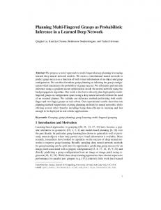
posterior over actions. It requires parameter optimization using Expectation Maximization (EM) which uses the inference machinery in an internal loop. Second, we formulated a probabilistic model that actually consists of a mixture of finite-length MDPs. This turned out to be very convenient to resolve a number of issues. All inference approaches, including ours, introduce a random variable to represent reward or success and condition this variable. However, when rewards can be collected at any time step in an infinite process it is unclear which future reward variable to condition (the issue of “somewhere in the future” we mentioned above). Conditioning reward random variables in each time step to observe reward does not lead to an equivalence to maximization of (discounted) expected future return (also a log-transformation does not help). The mixture of MDPs solves this issue. One could think of the mixture model as a superposition of possible world where in each one the reward event (the mental ice cream observation) is observed at another time T and its probability is proportional to some weighting γ T . We now do inference under this uncertainty of which world we live in. Since mixtures correspond to summation it almost trivially turns out that maximizing the reward likelihood in this mixture model is equivalent to the classical notion of maximizing the expected future return (sum of discounted rewards) in the MDP. In effect, we solved the problem of handling discounted total rewards in the inference framework and also found an efficient inference technique that probabilistically propagates forward from time zero and backward from the unknown time of the reward event. For further details we would like to refer to [35] and the extended version [36]. The resulting algorithm is an EM algorithm that yields optimal policies in an MDP. However, this first work is still a rather limited realization of the general concept. An MDP is a very strong abstraction of decision processes: every time slice contains only two random variables (a state variable st and an action variable at , coupled by a predictive model P (st+1 | at , st ) and the policy π(at | st )), graphically a0

a1

a2

s1

s2

π

s0

This is a strong simplification from the picture we have drawn in section 2, where the future is described by many random variables at each time, referring to various state features, abstractions, motor variables, or other representations. Further, in the simple MDP framework one can show very close similarity between the resulting EM algorithm and classical policy iteration – put critically, we introduced a rather fancy, complicated new theory only to end up with a well-known classical algorithm (though there are differences, e.g., w.r.t. exploiting the forward propagated messages). This equivalence to policy iteration indirectly also provides the proof of convergence to optimal policies, which is not obvious since EM-algorithms are only guaranteed to converge to local optima. However, in the developed framework it is rather straightforward to generalize the algorithm beyond the simple MDP case: e.g., to structured representations (more variables) and partial observability. In conclusion, the framework does not payoff much in the simple MDP case. But it is powerful to generalize to more interesting and harder problems, as we will see in the

n2 t

n2 t0

n1 t

n1 t0

n0 t

n0 t0

yt

st

at

y t0 st0

Figure 1: Partially observable Markov Decision Process with hierarchical controller. next section.

3.3

Hierarchical controllers and POMDPs

Partial observability means that we cannot observe the state directly. Formally, this introduces an additional random variable in our DBN: the observation yt we make in a certain time step which only encodes partial information about the true state of the environment. The interesting aspect about POMDPs (partially observable MDPs) is that a direct sensor-to-action association can usually not lead to optimal behaviors since the sensor information (yt ) is not sufficient to take optimal decisions. Instead, the agent needs some kind of internal memory or context representation that summarizes past observations and augments the current observation so that together they form a sufficient basis to take optimal decisions. One way to represent information that can be gained from past observation is to maintain the so-called belief – a distribution over the world state. This distribution contains all information that can be extracted from observations for making optimal decisions. We refer to other publications on belief-based approaches, e.g., [26]. In our work we followed another common approach. One assumes that the agent uses an internal automaton to process past and current observations and decide on an action. Usually a very simply structured automaton is assumed, a so-called FSC (finite state controller), which comprises a single internal state variable (or node) which changes its state depending on observations. A direct mapping from the internal state to actions realizes the decision-making. Generally, the agent’s internal automaton to process observations and build internal context representations may be much more complex. In [12, 6] hierarchical automata were proposed which contain not only one internal state variable but several variables on different levels; they are coupled as in typical hierarchical process models (like hierarchical Hidden Markov Models). These extended FSCs can represent hierarchical behaviors in a POMDP context, where a higher-level process controls a lower-level control process. For the scope of this paper the details of these hierarchical automata and the POMDPs are not important (see [37] for more details). What we described above means that we represent the future again as a DBN which now comprises much more variables than just states and actions. In graphical notation, the DBN we assume is given in figure 1. In each time step it comprises the (unobserved) environment state st , the observation

yt , the action at , and the hierarchy of internal states n0t ,..,n2t . The specific coupling structure can be exploited in the inference machinery (the maximal clique size in the Junction Tree Algorithm remains tractable also for many levels of hierarchies). In essence we are back to the general picture developed above: the future is spread out in terms of a DBN and we can use inference and Expectation Maximization to solve planning problems. In [37] we used this technique to solve POMDPs using hierarchical FSCs. The method significantly outperforms previous methods to optimizing hierarchical FSCs [6], in particular with increasing problem sizes. The complexity of the method fully depends on the cost of the inference query – the more structured the world or agent is, the more we can exploit this structure and use efficient inference techniques. On some large problems our method is also competitive to the state-of-the-art POMDP solver (HSVI2, heuristic search value iteration, [29]). We currently investigate even larger problems where the environment is structured (factored POMDPs) and hope to push the limits of what is solvable significantly further with the new technique.

3.4

Approximate inference for stochastic optimal control

The previous examples address problems in discrete domains. But the concept is in no way limited to discrete variables. Continuous and hybrid (mixed discrete and continuous) domains are naturally formalized in DBNs; a typical example for a hybrid DBN model are switching state-space models. See, e.g., [22] for more examples to include discrete and continuous variables in DBNs with appropriate couplings. In this section we want to demonstrate the inference approach on the level of motor control and planning – and suggest that the concept covers the whole spectrum between symbolic reasoning and sub-symbolic sensor-motor processing. A standard mathematical framework for motor control and planning is stochastic optimal control. In the standard case we assume we have a single state random variable qt that describes the physical state (posture and velocities) of articulated degrees of freedom, and a motor control variable ut . The physics of the system implies a stochastic process P (qt+1 | ut , qt ) (in discretized time). Again, the details of this stochastic model are not important for the scope of this paper – we refer to [34, 33] for more details. In essence, we again have a DBN as a spread out representation of the future, this time with variables qt and ut in each time step. A basic problem in motor planning is to reach a desired end posture at a desired point T in time. This rather literally translates to our picture of mentally observing ourselves to be in the desired posture at time T (conditioning the random variable qT to the desired posture) and then using the inference machinery to compute what this implies on all other variables – in particular the current motor control variable. Let us make this a bit more realistic: in typical motion problems the whole goal configuration is not specified, but only certain aspects of the posture, so-called task variables of the configuration. The most basic example is a 3-dimensional end-effector (e.g., hand) position, other examples for task variables are the collision state between objects (actually a discrete variable) or the balance (horizontal offset) over a point of support. In our DBN picture, all task variables are additional random variables that are coupled to the posture vari-

able qt in each time slice. A goal is specified, for instance, by reaching a certain 3D position with the end-effector at time T , not colliding and keeping balance in the time interval [0, T ]. All these goals and constraints can be expressed as conditioning the respective variables in the DBN. The inference machinery then computes estimates of intermediate postures and motor control variables that are coherent with all these constraints and goals. For the idea presented so far it is not clear to what degree the resulting control is optimal in the well-defined sense of stochastic optimal control. In fact, we have neglected a number issues in the simplified view above. For instance, classical stochastic optimal control usually assumes a cost term on the control variables – this can be be translated to a prior over the control variables in our DBN. Further, in the case of competing or contradicting constraints and goals, classical methods assume a task prioritization or a Tikhonov regularization to generate compromises [23]. In the DBN formulation this translates to certain non-tight couplings between qt and the task variables. In [33] we discuss in detail to what degree or in what sense the solutions found by approximate inference methods solve stochastic optimal control problems. The concrete approximate inference method we investigated is closely related to perturbative (variational) solutions around the optimal deterministic trajectory. Concerning the performance, we could demonstrate that the approximate inference techniques outperform stochastic optimal control solvers like iLQG [31], which is an efficient form of sequential quadratic programming. To give an impression of the performance, it takes about one second to compute a near-optimal posterior over a trajectory of length 200 for a 30 degrees-of-freedom robot in a reaching problem [33]. Similarly to our earlier work on MDPs, the work done so far on stochastic optimal control is limited to rather basic scenarios with only one state variable qt in the model. Although we can demonstrate good performance on these basic problems, the actual target are more complex structured problem like distributed or hierarchical motion planning problems on many concurrent and coupled variables. This is where the new approach should payoff even more since it can exploit structured inference methods – as in the POMDP case. Future research will have to examine this.

3.5

Extensions

Finally, let us briefly mention some recent extensions of the methods described in the previous sections. A model-free RL version. Although the focus of this paper is on planned behavior and model-based approaches, we also mention a recent derivation of a model-free RL algorithm from the idea of using inference for planning. Going back to the standard MDP case, we have shown in [35] that the problem of computing optimal policies can be translated to a problem of Expectation Maximization (EM) in a mixture of DBNs. From a theoretical point of view it is rather straight-forward to derive a model-free version of this method: inference can either be done by propagating exact messages (when we know the model in detail), or by sampling. It turns out that in the mixture of DBNs we can perform inference based on sampling which makes no explicit use of the model but only uses direct trajectory samples from the interaction with the environment. Since inference can be done

in a model-free way, also EM can be realized without model. In [39] we resorted to the SAEM algorithm (Stochastic Approximation EM) [9] as a theoretically well-grounded EM algorithm based on samples that guarantees convergence. Reasoning about the manipulation of objects. Our natural environment is composed of objects. The size of the state space grows exponentially with the number of objects (and their properties) and, when choosing inappropriate representations, inference methods become intractable. Artificial Intelligence research has from the beginning focused on better representations for worlds with objects by representing properties and relations using a logic framework. Recently there is increasing efforts to marry classical AI representations with the probabilistic framework and, in fact, it is possible to express and learn compact models of the environment in terms of probabilistic relational rules [40]. We took this representation as a starting point to develop methods that realize the use of inference in the case of worlds composed of objects [20]. With this approach we hope to capture the essence of the idea of internal simulation in the case of objects, i.e., the mental imagery of using and manipulating objects as a means to reach a goal. In its current form we developed an efficient inference machinery for this probabilistic rule-based representation, but still have to cope with extremely large representations since all objects are always taken into account. The next step will be to investigate more clever ways to reduce the computational burden, e.g., by focussing on only a subset of objects that seem relevant for the task.

4

Conclusion

In the previous section we presented a series of concrete realizations of the general idea, leading to different concrete algorithms when applied in the scope of MDPs, POMDPs, stochastic optimal control, or model-free RL. We hope that these examples make the overarching theme of using inference as a model for intelligent behavior more concrete and clear. In essence, we reduced the problem of planning, decision-making or motor control to a problem of inference on coupled sensor, motor and goal representations. At different places we pointed to analogies to the idea of internal simulation or mental imagery to organize goal-directed, prospective behavior. The key is to envision a possible future conditioned on reaching the goal – this envisioning can be set analogous to performing inference on possible futures conditioned on the “mental” observation of a goal. We believe that making connections to neuroscience and psychology, as we hinted at, is a particularly promising aspect of this approach – it would be most interesting to closely relate efficient and theoretically grounded methods of computer science to neuroscientific and psychological theories. First steps in this direction were already taken by Botvinick and An [2]. We would like to conclude with a discussion of a slightly more global view on the whole system. In standard approaches to, for instance, integrated robotic systems one typically discriminates between problems of sensor processing, motor control, behavior planning, etc. In terms of the system architecture one speaks of a modular design with black box algorithms that specialize on subtasks with well-defined interfaces and a well-defined flow

of information between them. Within each black box there are completely different and specialized algorithms and computational principles at work. Conceptually, the method we introduced suggests the exact opposite: The inference approach does not distinguish between the problems of sensor processing, motor control, or planning. The same information processing principle applies in all cases; in some sense, the computational mechanisms of inference treat all variables equal, no matter what the semantics of their representation is. There is no one-directional computational flow from sensor to motor; representations are coupled and a continuous recursive information exchange between all representations leads (hopefully) to convergence and posterior estimates of unobserved variables, be they perceptions, actions or motor signals. In practice, of course, this ideal of a generic information processing scheme that can solve all problems is too simplified. For inference methods to be efficient they need to use approximations that are specialized to the concrete representations and tasks. For instance, we used Gaussian belief representations to address stochastic optimal control problems – a crude but efficient approximation. Similar computational tricks are necessary to efficiently handle rule-based world models. Nevertheless, the conceptual idea of a generic computational principle to address seemingly diverse problems is interesting, also in view of the system design problems that are currently predominant in the development of integrated intelligent systems such as robots.

Acknowledgments This research was supported by the German Research Foundation (DFG), Emmy Noether fellowship TO 409/1-3.

References [1] H. Attias. Planning by probabilistic inference. In C. M. Bishop and B. J. Frey, editors, Proc. of the 9th Int. Workshop on Artificial Intelligence and Statistics, 2003. [2] M. Botvinick and J. An. Goal-directed decision making in prefrontal cortex: A computational framework. In Advances in Neural Information Processing Systems (NIPS 2008), 2009. in print. [3] C. Boutilier, T. Dean, and S. Hanks. Decision theoretic planning: structural assumptions and computational leverage. Journal of Artificial Intelligence Research, 11:1–94, 1999. [4] H. Bui, S. Venkatesh, and G. West. Policy recognition in the abstract hidden markov models. Journal of Artificial Intelligence Research, 17:451–499, 2002. [5] A. Cano, M. G´ omez, and S. Moral. A forward-backward monte carlo method for solving influence diagrams. Int. Journal of Approximate Reasoning, 42:119–135, 2006. [6] L. Charlin, P. Poupart, and R. Shioda. Automated hierarchy discovery for planning in partially observable environments. In NIPS, pages 225–232, 2006. [7] G. Cooper. A method for using belief networks as influence diagrams. In Proc. of the Fourth Workshop on Uncertainty in Artificial Intelligence, pages 55–63, 1988. [8] P. Dayan and G. E. Hinton. Using expectation maximization for reinforcement learning. Neural Computation, 9: 271–278, 1997.

[9] B. Delyon, M. Lavielle, and E. Moulines. Convergence of a stochastic approximation version of the EM algorithm. The Annals of Statistics, 27:94–128, 1999. [10] K. Doya, S. Ishii, A. Pouget, and R. P. N. Rao, editors. Bayesian Brain: Probabilistic Approaches to Neural Coding. MIT Press, 2007. [11] R. Grush. The emulation theory of representation: motor control, imagery, and perception. Behavioral and Brain Sciences, 27:377–396, 2004. [12] E. A. Hansen and R. Zhou. Synthesis of hierarchical finitestate controllers for pomdps. In ICAPS, pages 113–122, 2003. [13] G. Hesslow. Conscious thought as simulation of behaviour and perception. Trends in Cognitive Sciences, 6:242–247, 2002. [14] R. Howard and J. Matheson. Influence diagrams. In R. Howard and J. Matheson, editors, Readings on the Principles and Applications of Decision Analysis, volume II. Menlo Park CA: Strategic Decisions Group (1984), 1981. [15] F. Jensen, F. V. Jensen, and S. L. Dittmer. From influence diagrams to junction trees. In Proc. of the Tenth Conf. on Uncertainty in Artificial Intelligence, pages 367–373. Morgan Kaufmann, 1994. [16] A. Johnson and A. Redish. Neural ensembles in CA3 transiently encode paths forward of the animal at a decision point. J. Neuroscience, 27:12176–12189, 2007. [17] M. I. Jordan. Learning in graphical models. MIT Press, Cambridge MA, 1999. [18] U. B. Kjaerulff and A. L. Madsen. Bayesian Networks and Influence Diagrams: A Guide to Construction and Analysis. Information Science and Statistics. Springer, 2008. [19] Kschischang, Frey, and Loeliger. Factor graphs and the sum-product algorithm. IEEE Transactions on Information Theory, 47, 2001. [20] T. Lang and M. Toussaint. Approximate inference for planning in stochastic relational worlds. In Proc. of the 26rd Int. Conf. on Machine Learning (ICML 2009), 2009. [21] A. Madsen and F. Jensen. Solving linear-quadratic conditional gaussian influence diagrams. Int. Journal of Approximate Reasoning, 38:263–282, 2005. [22] K. Murphy. Dynamic bayesian networks: Representation, inference and learning. PhD Thesis, UC Berkeley, Computer Science Division, 2002. [23] Y. Nakamura, H. Hanafusa, and T. Yoshikawa. Taskpriority based redundancy control of robot manipulators. Int. Journal of Robotics Research, 6, 1987. [24] T. Ott and R. Stoop. The neurodynamics of belief propagation on binary markov random fields. In Advances in Neural Information Processing Systems (NIPS 2006), volume 19, pages 1057–1064. MIT Press, 2007. [25] J. Pearl. Probabilistic Reasoning In Intelligent Systems: Networks of Plausible Inference. Morgan Kaufmann, 1988. [26] J. Pineau, G. Gordon, and S. Thrun. Anytime point-based approximations for large POMDPs. Journal of Artificial Intelligence Research, 27:335–380, 2006. [27] T. Raiko and M. Tornio. Learning nonlinear state-space models for control. In Proc. of Int. Joint Conf. on Neural Networks (IJCNN 2005), 2005. [28] R. D. Shachter. Probabilistic inference and influence diagrams. Operations Research, 36:589–605, 1988.

[29] T. Smith and R. G. Simmons. Heuristic search value iteration for pomdps. In UAI, pages 520–527, 2004. [30] R. Sutton and A. Barto. Reinforcement Learning. MIT Press, Cambridge, 1998. [31] E. Todorov and W. Li. A generalized iterative lqg method for locally-optimal feedback control of constrained nonlinear stochastic systems. In Proc. of the American Control Conference, pages 300–306. 2005. [32] M. Toussaint. Lecture notes: Factor graphs and belief propagation. http://ml.cs.tu-berlin.de/˜mtoussai/notes/, 2008. [33] M. Toussaint. Robot trajectory optimization using approximate inference. In Proc. of the 26rd Int. Conf. on Machine Learning (ICML 2009), 2009. [34] M. Toussaint and C. Goerick. Probabilistic inference for structured planning in robotics. In Int Conf on Intelligent Robots and Systems (IROS 2007), pages 3068–3073, 2007. [35] M. Toussaint and A. Storkey. Probabilistic inference for solving discrete and continuous state Markov Decision Processes. In Proc. of the 23nd Int. Conf. on Machine Learning (ICML 2006), pages 945–952, 2006. [36] M. Toussaint, S. Harmeling, and A. Storkey. Probabilistic inference for solving (PO)MDPs. Technical Report EDIINF-RR-0934, University of Edinburgh, School of Informatics, 2006. [37] M. Toussaint, L. Charlin, and P. Poupart. Hierarchical POMDP controller optimization by likelihood maximization. In Uncertainty in Artificial Intelligence (UAI 2008), 2008. [38] D. Verma and R. P. N. Rao. Goal-based imitation as probabilistic inference over graphical models. In Advances in Neural Information Processing Systems (NIPS 2005), 2006. [39] N. Vlassis and M. Toussaint. Model-free reinforcement learning as mixture learning. In Proc. of the 26rd Int. Conf. on Machine Learning (ICML 2009), 2009. [40] L. Zettlemoyer, H. Pasula, and L. P. Kaelbling. Learning planning rules in noisy stochastic worlds. In Proc. of the Twentieth National Conf. on Artificial Intelligence (AAAI 05), 2005. [41] N. L. Zhang. Probabilistic inference in influence diagrams. Computational Intelligence, 14(4):475–497, 1998.

Marc Toussaint is head of the Emmy Noether research group on “Machine Learning and Robotics” at TU Berlin since 2007. Before this, he spend two years as a post-doc at the University of Edinburgh with Prof. Chris Williams and Prof. Sethu Vijayakumar, and received his PhD in 2004 at the Ruhr-University Bochum. His recent focus of research is in Machine Learning methods, in particular probabilistic inference methods, and their application in context of goal-directed behavior and robotics.