National University of Singapore, Kent Ridge, Singapore 119260. Abstract: Many process characteristics follow exponential distribution and control charts.
Appeared in: Journal of Applied Statistics, 2000, 27, 1050-1063.
Process Monitoring of Exponentially Distributed Characteristics Through an Optimal Normalizing Transformation
Zhenlin Yang Department of Statistics and Applied Probability National University of Singapore, Kent Ridge, Singapore 119260
Min Xie Department of Industrial and Systems Engineering National University of Singapore, Kent Ridge, Singapore 119260
Abstract: Many process characteristics follow exponential distribution and control charts based on such a distribution have attracted a lot of attention. Traditional control limits may be not appropriate because of the lack of symmetry. In this paper, process monitoring through a normalizing power transformation is studied. The traditional individual measurements control charts can be used based on the transformed data. The properties of this control chart are investigated. Comparison with the chart using probability limits is also carried out for the cases of known and estimated parameter. Without losing much accuracy even compared with the exact probability limits, the power transformation approach can easily be used to produce charts that can be interpreted when the normality assumption is valid.
Appeared in: Journal of Applied Statistics, 2000, 27, 1050-1063.
2
1. Introduction A basic assumption in using the traditional Shewhart-type control charts is that the quality characteristic involved follows a normal distribution. The Shewhart charts may still be applicable to non-normal situations when the sample size is large as guaranteed by the Central Limit Theorem. However, in modern manufacturing environment, items are often checked one by one and control charts for individual measurements are desirable, see e.g., Sheil (1995), Gong et al. (1997) and Xie et al. (1998). The normality assumption for individual value is usually questionable and the normality should be tested before the implementation of traditional technique. In case the normality is rejected, it can be convenient to first transform a non-normal variable to near normal and then apply the traditional control charts on the transformed values. In this paper, process monitoring for exponentially distributed quality characteristic is discussed and properties for such a chart based on transformation are studied. One usefulness of a control chart for the exponential measurement is that it can be used as a control chart for parts-per-million nonconforming items (Nelson, 1994 and Radaelli, 1998). The idea is that if the number of nonconforming items is assumed to be a Poisson random variable then the 'time' until a defective item has an exponential distribution. Usually this 'time' can be real time, length or volume, etc. If the production process has a constant speed, then obviously the count and the time until a defective item are equivalent quantities (Nelson, 1994) that can both be modeled by an exponential distribution. Nelson (1994) proposed a normalizing transformation which may be not an optimal(*) one and the properties of the chart based on this transformation have not been investigated. A control chart based on an optimal normalizing transformation is proposed
(*)
It should be noted that the “optimality” depends on the adopted “optimality” criterion.
Appeared in: Journal of Applied Statistics, 2000, 27, 1050-1063.
3 in this paper. The property of this chart is investigated. At the same time it is compared with the chart for exponential distribution with probability limits. Both the case of known parameter and estimated one are discussed. The investigation or comparison for parameter unknown case are done via an extensive Monte Carlo simulation. This paper is organized as follows. Section 2 discusses the best transformation within the power family. Section 3 investigates the properties of the control charts when the model parameter is known, whereas Section 4 considers the case of unknown parameter where extensive Monte Carlo simulation results are presented. Two illustrative examples are also presented in Section 5.
2. The Best Normalizing Power Transformation 2.1. Background In studying the large sample behavior of transformations to normality, Hernandez and Johnson (1981) considered an information number approach to transform a known distribution to near normality, to serve as benchmarks for the maximum amount of improvement achievable through Box-Cox transformation (Box and Cox, 1964). The Box-Cox transformation technique aims to transform the nonnegative data to near normal through a simple power transformation so that the normal theory procedures can be applied to the transformed data. It is seen to have many applications in reliability, quality control and lifetime data analysis. See for example, Hinkle and Emptage (1991), Fearn and Nebenzahl (1995) and Yang (1999). Let the probability density function (pdf) of a continuous nonnegative random variable X be g ( x; ) where is the mean. Denote by Y = X the power transformed
observation and f ( y; , ) its pdf. Let ( y; , ) be a normal pdf with mean and standard deviation (SD) . The basic idea of finding the `best` normalizing transformation
Appeared in: Journal of Applied Statistics, 2000, 27, 1050-1063.
4 is to find , and such that f ( y; , ) and ( y; , ) are closest in a certain sense. Hernandez and Jonhson (1981) suggested the so-called Kullback-Leibler (KL) information number as a measure of closeness:
I ( f , ) =
f ( y; , )
f ( y; , ) log ( y; , ) dy .
(2.1)
0
Thus, the optimal transformation value 0 is found by minimizing (2.1). That is, minimize I [ f (; , ), (; , )] over (, , ).
(2.2)
This can be done by using the general result of Hernandez and Johnson (1981). For an exponential distribution, a direct algebraic manipulation can be easier. 2.2. Derivation of the best power transformation for exponential variables
If X is an exponential random variable, then its pdf has the form g ( x; ) =
1 exp( x ) , > 0. The pdf of Y = X is thus f ( y; , ) = ( ) 1 y 1 1 exp( y 1 ) by change of variable technique. Indeed, it can be noticed that f ( y; , ) is a Weibull pdf of the form y 1 exp[( y ) ] with = 1 and = . If ( y; , ) is a normal pdf with mean and SD , then the Kullback-Leibler information between f ( y; , ) and
( y; , ) becomes
I ( f , )
=
0
1 1 1 y1 log y exp
1
2 1 = log + 2
0
y 1 1 exp( 1 y 1 ) dy 2 1 1 exp 2 ( y ) 2 2 1
y 1 1 log y exp 1 y 1 dy
1 1 y 2 1 1 y 1 1 ( y ) 2 exp 1 y 1 dy 2 0
2
Appeared in: Journal of Applied Statistics, 2000, 27, 1050-1063.
5 By introducing x y 1 , the first integral becomes
0
y1 1 log y exp 1 y1 dy =
0
2 log x exp 1 x dx = 2 (log ) ,
where =0.577216, the Euler-Gamma constant and the second integral becomes
0
=
0
1 y
2 1
1 x
1 2 y 1 1 ( y ) 2 exp 1 y 1 dy 2
1
2 2
x 2
2 x 2 exp 1 x dx 2 2
2 = 2 (2 1) 2 1 + 2 ( 1) 1 2 . 2
2
Finally, we have 2 2 I ( f , ) = log + (1)(log) 1 + 21 2 (2 1) 2 2 ( 1) + 2 2 .
Now, setting the partial derivatives of I ( f , ) with respect to and to zero and solving the equations, it can be shown that I ( f , ) is partially minimized at
() = ( 1) and 2 ( ) = 2 [(2 1) 2 ( 1)] . Substituting () and 2 ( ) back into I ( f , ) gives the partially minimized KullbackLeibler information number I() = 12 log(2 ) + (1) 12 log + 12 log[ (2 1) 2 ( 1) ].
Finally, minimizing I() gives the best transformation. This can be done by any of numerical maximization procedure. The resulted optimal parameter values are:
0 = 0.2654, 0 = 0.9034 and 0 = 0.2675 0
0
Appeared in: Journal of Applied Statistics, 2000, 27, 1050-1063.
6 and the minimized distance is I [ f (; , 0 ), (; 0 , 0 )] = 0.00278.
Notice that I() is independent of the parameter , which makes the transformation very attractive to the practitioners. It is interesting to point out that the original exponential pdf ( = 1), having a KL number of 0.4189, is very 'far' from a normal pdf. Comparison of the minimized KL information numbers shows therefore a great improvement to normality by such a simple power transformation. It can be further noted that using the power transformation proposed in Nelson (1994), by matching the first few moments, = 0.2777, we have a KL number of 0.00293, that is approximately 5% larger than that from the transformation 0 = 0.2654, showing that = 0.2777 is not optimal in terms of KL minimizing criterion. Hence, although the two transformations perform similarly, the former is recommended as it has a sound theoretical basis. Table 2.1 presents some tail probabilities of the optimally transformed Y with the related normal variable. It has seen that the tail probabilities of Y are very close to those of the corresponding normal random variable.
Table 2.1. Tail Probabilities for the Transformed Exponential Random Variable K 0.5 1.0 1.5 2.0 2.5 3.0 P (Y 0 k 0 ) 0.311204 0.166061 0.071875 0.022950 0.004234 0.000176 P (Y 0 k 0 ) 0.317539 0.163359 0.065652 0.019569 0.004089 0.000564 Normal Tail Prob. 0.308538 0.158655 0.066807 0.022750 0.006210 0.001350
Appeared in: Journal of Applied Statistics, 2000, 27, 1050-1063.
7
3. Control Chart when is Known In this section the operating characteristic (OC) function of the chart for Y is investigated for the case when the in-control exponential mean, , is known and compared with the chart for X based on the exact probability limits. It should be pointed out that for asymmetrically distributed characteristics the exact probability limits should be usually preferable to the traditional 3-sigma limits. Indeed, it can be noted that for the exponential distributions, 3-sigma limits would lead to a negative LCL. The two-sided control chart for the original X, with allowed false alarm probability or Type I risk is of the form: LCL = log(1 2) , CL = 0.6931 ,
(3.1)
UCL = log( 2) .
In accordance with the usual approach, the two-sided control chart for Y can be defined as follows: LCL = 0 k 0 , CL = 0 ,
(3.2)
UCL = 0 + k 0 ,
where 0 =0.9034 0.2654 , 0 =0.2675 0.2654 and k is the number of SDs allowed in the control limits. The ability to detect shifts in process quality is an important factor to be considered in designing a control chart. Such ability is often measured by the OC function of the control chart, which is defined as the probability of not detecting a shift under an out-ofcontrol situation. This probability represents the type II risk . As we are interested in
Appeared in: Journal of Applied Statistics, 2000, 27, 1050-1063.
8 detecting a shift in exponential mean , the -risk for an r SDs shift in the mean of X is given (under the X chart) by
X (r ) = P 0 log(1 2 ) X 0 log(2 ) 0 r 0
(3.3)
= (1 2) 1 (1 r ) ( 2)1 /(1 r ) . For the Y chart, the OC function is:
Y (r ) = P 0 k 0 Y 0 k 0 0 r 0 0.9034 0.2675k = exp 1 r
1 0
0.9034 0.2675k exp 1 r
1 0
,
(3.4)
where k > 0 is so that PY 0 k 0 + PY 0 k 0 = . Notice that one SD shift in X scale causes less than one SD shift in Y scale. The X chart centers at the median position while the Y chart centers at the mean position. This is not unexpected since the distribution of Y is almost symmetric, with mean and median almost the same, which are 0.9034 0 and (0.6931 ) 0 = 0.9073 0 , respectively. Figure 3.1 shows the OC function of X and Y charts, for two typical values of k, i.e., k = 2 (equivalently = 0.0455) and k = 3 ( = 0.0027).
b risk , k=2
b risk , k=3
1 0.8 0.9 0.6 0.8
0.4
0.7
0.2 0 -1
0
1
2
3
4
5
6
-1
0
1
2
3
4
Figure 3.1. OC Curves for X chart (solid line) and Y chart (dashed line).
5
6
Appeared in: Journal of Applied Statistics, 2000, 27, 1050-1063.
9 As expected, for k =2 two charts perform very similarly, whereas for k = 3 the exact probability limits will perform slightly better than the transformed Y chart. However, the chart based on the transformation is able to provide a similar level of sensitivity, especially for the case of small to medium shift. Lastly, it can be remarked that, as is known, comparison between the Average Run Lengths (ARLs) of X and Y charts is readily derivable from the OC curves.
4. Control Chart when is Unknown When is unknown, it can be commonly estimated on earlier process data. In this case, the properties of the two charts are not obvious. In this section, the two approaches are compared for the case that is unknown and supposed to be estimated from n past observations X1, X2, …, Xn. 4.1. Derivation of the control limits
For the X chart, the sample mean X can be used to estimate , which gives the X chart with estimated control limits: LCL*X X log(1 2) , CL*X 0.6931X ,
(4.1)
UCL*X X log( 2) .
For the Y chart, one can work directly with the transformed data and construct a control chart in the usual way as if the transformed data are exactly normal. A typical control chart would be the one which uses the mean of past data as an estimator or 0 and the mean of the moving ranges as an estimator of 0 (Nelson, 1994):
Appeared in: Journal of Applied Statistics, 2000, 27, 1050-1063.
10 LCL*Y Y k MR2 d 2 , CL*Y Y ,
(4.2)
UCL*Y Y k MR2 d 2 . where MR 2 is the mean of the moving ranges of two observations and d 2 = 1.128. There are other ways to estimate the control limits of the Y chart. However, we will focus our study on (4.2) as it is more common for individual chart that is the case here. 4.2. Comparison of the alarm rate
Since the control limits are estimated in this case, it is difficult to evaluate the -risk, the -risk and the ARL. Monte Carlo simulation is helpful and convenient for the investigations. There are three issues that have to be addressed for the Y chart with estimated control limits: i) the effect of nonnormality as the transformed data are still not exactly normal, ii) the effect of estimated control limits, and iii) the relative performance compared with the X chart. As the comparison of the Y chart with X chart is the aim of this paper, we will concentrate on the last issue. The simulation process can be simply described as follows. Let Bi be the event that the next ith observation falls either below LCL* or above UCL* . Then P( Bi ) represents the probability that the next ith observation signals a
process out of control. When process is in control, P( Bi ) is the -risk while when the process is shifted, then 1P( Bi ) is the -risk. Notice that in contrast to the known control limit case, the Bi 's are not independent anymore. Hence the ARL does not equal to 1/ or 1/(1). We first simulate P( Bi ) and then ARL for certain values of n and r.
Appeared in: Journal of Applied Statistics, 2000, 27, 1050-1063.
11 To simulate P( Bi ) for the X chart, n values from Exp() are generated to calculate
LCL*X and UCL*X . Then a value from Exp(+ r) is generated and is counted by one if this value is either below LCL*X or above UCL*X . Repeat this process many times. The proportion of times that the extra value falls either below LCL*X or above UCL*X gives a Monte Carlo estimate of P( Bi ). To simulate P( Bi ) for the Y chart, generate n values from Exp(), raise these values to a power of 0 , and then calculate LCL*Y and UCL*Y . Generate another value from Exp(+ r), and raise it to a power of 0 , and then check to see if this value falls below
LCL*Y or above UCL*Y . Repeat this process many times. The proportion of times that the extra value falls outside of the control limits gives a Monte Carlo estimate of P( Bi ) for the Y chart. All the simulation results in this paper were based on 100,000 runs, that ensured a good accuracy of the simulated probabilities. For example, the estimated standard error of the estimated probability 0.002 is only 0.000141. Some results are presented in Table 4.1. It can be seen that the alarm rate is similar for both methods. Table 4.1. Simulated probabilities of acceptance at r sigma shift
Upper entry is for the X chart; lower entry is for the Y chart. r=-0.8
n = 20 50 100
n = 20 50 100
-0.5
0.8923 0.8516 0.8914 0.8738 0.8922 0.8844
0.9543 0.9309 0.9539 0.9454 0.9543 0.9514
0.9933 0.9784 0.9934 0.9929 0.9931 0.9963
0.9972 0.9912 0.9972 0.9968 0.9973 0.9986
0.0 1.0 2.0 k = 2 = 0.0455) 0.9465 0.8254 0.7011 0.9347 0.8291 0.7144 0.9510 0.8336 0.7037 0.9490 0.8444 0.7188 0.9534 0.8363 0.7070 0.9541 0.8470 0.7228 k = 3 ( = 0.0027) 0.9951 0.9531 0.8759 0.9912 0.9571 0.8943 0.9969 0.9586 0.8840 0.9975 0.9694 0.9092 0.9969 0.9613 0.8867 0.9982 0.9731 0.9150
3.0
4.0
5.0
6.0
0.5976 0.6142 0.6039 0.6225 0.6035 0.6215
0.5186 0.5384 0.5221 0.5401 0.5247 0.5435
0.4566 0.4768 0.4632 0.4809 0.4620 0.4791
0.4102 0.4299 0.4122 0.4302 0.4172 0.4335
0.7963 0.8275 0.8014 0.8391 0.8040 0.8437
0.7226 0.7620 0.7288 0.7722 0.7278 0.7728
0.6568 0.7023 0.6638 0.7118 0.6674 0.7167
0.6024 0.6517 0.6053 0.6546 0.6102 0.6584
Appeared in: Journal of Applied Statistics, 2000, 27, 1050-1063.
12 4.3. Comparison of the ARL
Unlike the case of a known , the ARL cannot be easily calculated as the events Bi 's are no longer independent. Monte Carlo simulation is used here. To obtain the ARL, n values with zero shift from the target value are generated to calculate the estimated control limits. Then a number of values are generated with an r sigma shift from the target value, until an out of control signal is given. This number serves as one observation drawn from the run length distribution. Repeat this process many times. The mean of all the observations drawn from the run length distribution serves as an estimate of the ARL. Since the original measurements are exponential and the transformed measurements are Weibull where both cases give closed form cdfs, it is possible to give an equivalent but simpler algorithm for simulating ARL. Instead of generating additional measurements at the shifted mean until one out of control signal, we can simply generate a geometric observation with the probability of success (out of control) being the conditional probability that a new observation is out of the estimated control limits. For the X chart, it is
p = P ( X 0 LCL*X X) P( X 0 UCL*X X) LCL*X = 1 exp (1 r ) 0
UCL*X exp (1 r ) 0
,
and for the Y chart, it is given by
p = P (Y 0 LCL*Y Y) P(Y 0 UCL*Y Y)
( LCL*Y )1 0 = exp (1 r ) 0
(UCL*Y )1 0 exp (1 r ) 0
where X and Y denote the original and transformed vectors of past observations. Notice that to calculate p for the Y chart, it is necessary that LCL*Y be nonnegative. This is not always true for the Y chart using MR .
We thus use the Y chart with ˆ X for
Appeared in: Journal of Applied Statistics, 2000, 27, 1050-1063.
13 simulation and comparison. The simulated ARLs are summarized in Table 4.2. Again, each simulated ARL is based on 100,000 runs. In this case, it can be found that all the estimated standard errors are around 0.4% of the corresponding simulated ARLs, showing that the simulated ARLs are very accurate. Table 4.2. Simulated ARLs: Upper entry is for X chart; lower entry is for Y chart. r=-0.8 n = 20 50 100
n = 20
9.64 9.62 9.37 9.31 9.28 9.25
-0.5 22.11 22.02 22.09 22.11 22.19 21.96
156.42 380.75 1189.47 2834.75 50 152.24 377.35 1158.46 2861.14 100 149.98 375.08 1148.80 2844.56
0.0 k = 2 20.52 21.83 21.39 22.67 21.61 23.10 k = 3 330.09 1529.13 350.84 1486.41 359.23 1443.02
1.0 2.0 3.0 ( = 0.0455) 6.53 3.54 2.58 7.00 3.73 2.70 6.32 3.50 2.55 6.75 3.66 2.67 6.24 3.45 2.54 6.66 3.64 2.64 ( = 0.0027) 34.75 10.20 5.60 61.22 14.26 7.09 29.82 9.44 5.36 48.64 12.86 6.71 28.00 9.22 5.28 44.95 12.50 6.62
4.0
5.0
6.0
2.14 2.21 2.12 2.19 2.12 2.19
1.89 1.93 1.87 1.93 1.87 1.92
1.72 1.75 1.71 1.75 1.71 1.74
3.90 4.74 3.81 4.55 3.77 4.51
3.10 3.62 3.04 3.53 3.03 3.53
2.64 3.00 2.60 2.94 2.58 2.93
From Table 4.2 we see that, for k = 2 ( = 0.0455) and when the process is in control (r = 0), the ARLs for both charts are all very close to the nominal value 1/ = 1/.0455 = 21.98, though the values for the Y chart are slightly larger. When there is a shift in the process mean, the ARLs for the X chart and Y chart are again very close, showing that the two charts are essentially equivalent in detecting a process shift. Also from Table 4.2, for the charts with = 0.0027 or k = 3, the Y chart has much larger ARLs than the X chart when process is in control, which is not bad. For relatively small shifts the Y chart leads to a larger out-of-control ARL than the X chart (e.g., for n = 100 and r = 3, Y-ARL was approximately 25% larger than the X-ARL). However, when there is a large enough shift in process mean, the ARLs for the two charts are very close, meaning that the power transformation-based chart will be able to detect process shift at a comparable fast speed to the original X chart (e.g., for n = 100 and r = 6, Y-ARL was approximately only 13% larger than the X-ARL).
Appeared in: Journal of Applied Statistics, 2000, 27, 1050-1063.
14
5. Two Implementation Examples In this section, two examples are used to illustrate the control charts discussed above. The first example uses a simulated data set for illustrating the known case and the second uses a real data set of Baker (1996) for illustrating the unknown case. Example 5.1. The simulated data. The first 30 values are generated from an exponential population with = 10 and used in deriving control limits, assuming = 0.0027 (i.e., k = 3). The next 20 values are generated from an exponential population with = 30 and the last 20 with = 50. The simulated data are listed below and the control charts are given in Figures 5.1 where the observations are plotted on the chart in the same order as they are listed in the table. Table 5.1. A set of simulated data. = 10 3.678 14.985 0.199
5.071 0.865 2.665 31.648 0.589 13.219
0.863 0.149
48.736 73.381 16.438 42.033
30.042 13.380 11.776 1.313 5.128 0.518
3.317 7.442 9.261 20.668 0.598 14.661
11.140 5.786 7.428 19.834 2.408 0.732
11.683 21.223 5.677
23.543 4.823 7.259 14.300 135.508 0.895 2.421 66.695 52.075 19.376 16.974 60.683
23.334 0.498
= 30 = 50
20.108 54.567 294.152 1.068 52.832 54.063 14.668 27.902 46.721 23.642 61.648 80.148 58.981 53.652
16.530 26.465
6.785 1.385 9.470 207.671
From the original X chart, we see that the plotted points cluster between LCL and CL which are very close to each other. This makes the data visualization difficult. From the control chart for the transformed data, we see that the plotted points scatter evenly around the center line. The two charts perform similarly as far as the ability of identifying a process shift is concerned, but the latter is easier to interpret. In fact, suppose that run rules and other tests (Nelson, 1984 and Wang et al., 1998) are to be implemented, it is much clearer if the transformed plot is used.
Appeared in: Journal of Applied Statistics, 2000, 27, 1050-1063.
15 1
300
X Chart Individual Value
1 200 1 100 UCL=66.0765 CL=6.9310 LCL=0.0135
0 0
10
20
30
40
50
60
70
Observation Number 5
1
Y Chart
1
Individual Value
4 UCL=3.1431
3
2 CL=1.6645 1 LCL=0.1859
0 0
10
20
30
40
50
60
70
Observation Number
Figure 5.1. Control charts for the simulated data
Example 5.2. The interfailure time data. The data set given in Table 5.2 represents the interfailure times for 92 successive failures of a photocopier system. It was originally given in Baker (1996) in the form of age (in days) at the failures. Table 5.2. A set of interfailure time data 7
1
1
49
26
2
12
6
0
8
1
6
2
6
0
67
1
17
4
13
0
1
36
1
12
13
8
1
7
9
7
11
2
15
32
9
18
8
42
9
5
7
23
4
18
6
19
3
6
0
14
12
16
19
8
5
4
7
5
0
22 11
8
1
2
3
11
3
2
8
9
11
26
63
37
7
50
12
3
3
3
6
2
3
36
20
64
22
9
17
10
0
Appeared in: Journal of Applied Statistics, 2000, 27, 1050-1063.
16 The likelihood ratio test (Lawless, 1982, p441) is performed on the original as well as the transformed data and the results are consistent with the hypothesized distributional assumptions. The sample mean of the original data is X =12.337. With = 0.0027 and k = 3, the control charts specified by (4.1) and (4.2) can be easily constructed, see Figure 5.2. It can be seen that the plotted points in Y chart scatter evenly on both sides of the centre line and again further interpretations are straightforward.
90 UCL=81.5186
80 1
70
Individual Value
X Chart 1
1
60 1
1
50 40 30 20 10
CL=8.5508
0
LCL=0.0167 0
10
20
30
40
50
60
70
80
90
100
Observation Number 4 UCL=3.5570 Y Chart
Individual Value
3
2 CL=1.6767 1
0 LCL= -0.2034 0
10
20
30
40
50
60
70
80
90 100
Observation Number
Figure 5.2. Control charts for the interfailure time data
Appeared in: Journal of Applied Statistics, 2000, 27, 1050-1063.
17
6. Conclusions The Box-Cox transformation can be used to transform a non-normal distribution to normal. In this paper, we have studied the use of this transformation for exponentially distributed quality characteristic by minimizing the Kullback-Leibler information number. The study indicates that it is easy to use and possesses a number of interesting statistical properties, especially it is of great advantage that the transformation to normality does not depend on the specific parameter value of the exponential distribution. Similar transformations have been proposed in Nelson (1994) and Kittlitz, Jr. (1999), but they may not be optimal and no investigation has been given for the properties of the resulted control charts. Compared with the traditional probability limits, the data transformation approach leads to a chart that is only a little less accurate than the exact one. The transformed data should be used when a control chart is to be interpreted in a traditional sense and especially when run rules are to be used. This is especially the case when the model parameter is unknown. However, it should be pointed out that data transformation approach should be avoided when plotting actual observation for data recording is an important issue for specific implementation.
Acknowledgement: The authors are grateful to the editor and to the referee for the detailed comments that lead to a significant improvement in the presentation of the paper. Part of this research is funded by a research grant from the National University of Singapore for the project “Some practical aspects of SPC for automated manufacturing process” (RP3981625).
Appeared in: Journal of Applied Statistics, 2000, 27, 1050-1063.
18
References Baker, R. D. (1996) Some new tests of the power law process. Technometrics, 38, 256265. Box, G. E. P. and Cox, D. R. (1964) An analysis of transformation (with discussion). Journal of the Royal Statistical Society B, 26, 211-252. Fearn, D.H. and Nebenzahl, E. (1995) Using power-transformations when approximating quantiles. Communications in Statistics - Theory and Methods, 24, 1073-1093. Gong, L.G., Jwo, W.S. and Tang, K. (1997) Using on-line sensors in statistical process control. Management Science, 43, 1017-1028. Kittlitz, Jr., R.G., (1999) Transforming the exponential for SPC applications. Journal of Quality Technology, 31, 301-308. Hernandez, F. and Johnson, R.A. (1981) The large-sample behavior of transformations to normality. Journal of the American Statistical Association, 75, 855-861. Hinkle, A.J. and Emptage, M.R. (1991) Analysis of fatigue life data using Box-Cox transformation. Fatigue and Fracture of Engineering Materials and Structures, 14, 591-600. Lawless, J. F. (1982) Statistical Models and Methods for Lifetime Data. John Wiley & Sons. New York. Nelson, L.S. (1984) The Shewhart control chart - tests for special causes. Journal of Quality Technology, 16, 237-239. Nelson, L.S. (1994) A control chart for parts-per-million nonconforming items. Journal of Quality Technology, 26, 239-240. Radaelli, G. (1998) Planning time-between-events Shewhart control charts. Total Quality Management, 9, 133-140. Sheil, J. (1995)
An economic-approach towards using individual measurements to
control the mean of continuously monitored processes. International Journal of Production Research, 33, 2959-2971.
Appeared in: Journal of Applied Statistics, 2000, 27, 1050-1063.
19 Wang, J.M., Kochhar, A.K. and Hannam, R.G. (1998) Pattern recognition for statistical process control charts. International Journal of Advanced Manufacturing Technology, 14, 99-109. Xie, M., Goh, T.N. and Lu, X.S. (1998).
Computer-aided statistical monitoring of
automated manufacturing processes. Computers and Industrial Engineering, 35, 189192. Yang, Z. (1999) Predicting a future lifetime through Box-Cox transformation. Lifetime Data Analysis, 5, 265-279.