European Journal of Scientific Research ISSN 1450-216X / 1450-202X Vol. 149 No 4 July, 2018, pp. 376-384 http://www. europeanjournalofscientificresearch.com
Proposed Algorithm to Solve Inverse Kinematics Problem of the Robot Hayder Fadhil Abdulsada Najaf Technical Institute, Al-Furat Al-Awsat Technical University 31001 Al-Najaf, Iraq E-mail:
[email protected] Abstract The problem of the Inverse kinematics (IK) of robot "manipulators" is desired to be treated analytically to have simply and completely solution. This operationis nameda closed method solution. In this paper, a proposed algorithm isutilized to overcome the IK and measure the angles of the arm's joints when they followto any track. The QNN algorithm is proposed to improve the system response and overcome the trouble of robot'sIK. Theforward kinematic (FK) was derived basing on the"Denavit-Hartenberg" representation. The system is simulated by Matlab-2014,the GUI is designed and built for the purpose of robotsimulations in FK, IK and in the movement path. In this implementation, a Mitsubishi-RM501 robot of 5 degrees of freedom was used. Keywords: "Denavit-Hartenberg", DOF, Forward Kinematic (FK), Inverse Kinematics (IK), QNN. 1. "The Mitsubishi-RM501" Robot System The M.RM501 robot isdescribed as a5 degree robot which has an effector-gripper that has openedand closed end. The robot has 3essential joints which are explained as following:"Base", "Shoulder" and "Elbow", the orientation (wrist) joints are "Pitch", "Yaw" and "Roll". Figure (1) shows a picture of the M.RM501 manipulator robot. The actuators of the robot are DC servo motors with different powers.For each joint, a sensor is attachedfor calculatingof the angular movement at the end of the joint(M. W. Spong et al, 2005). The characteristics of the Mitsubishi-RM501 robot systemareexplained in Table 1 below. Table 1:
The Mitsubishi-RM501characteristics
Join "Base" "Shoulder" "Elbow" "Wrist"
Link Length (mm) 250 220 160 65
Max. Rotation (Deg.) 300 130 90 ±180
Encoder steps 48400 21450 15371 39543
377
Hayder Fadhil Abdulsada Figure 1: Mitsubishi-RM501robot
2. Kinematics of Robotic Manipulators Robot's kinematics means the studying of the robots' motion. Regardless of the forces that caused this motion, the acceleration, velocity, and position, of all the links in a kinematics can be analyzed and calculated (Romdhane, and Duffy, 1991).The robot kinematicsincludeFK and IK. Theaim of the FK is to obtainthe endــeffector position in the space where the motions of its joints are known asFሺθଵ , θଶ , θ୬ ሻ = ["x, y ,z ,R"].The aim of the IK is findingthe joint variables that matchthespecified endــeffector location and orientationas "Fሺx, y, z, Rሻ" = θଵ , θଶ , … θ୬ . (Duffy, 1980). Figure 2: Kinematicsblock diagram(Denavit and Hartenberg, 1955)
3. FK Problem of M.RM501 Robot A techniqueof Denavit-Hartenberg (D-H) will be applied to solvetheFK ofthe MitsubishiRM501Robot.The parameters for Mitsubishi-RM501robot are illustratedin Table 2. Table 2:
(D.H) parameters ofMitsubishi-RM501 robot
Frame 1 2 3 4
a 0 220 mm 160 mm 0
α 90 0 0 90
d 250 mm 0 0 0
θ θ1 θ2 θ3 θ4
The FK describes the transformation from one frame to another, beginning from the base of effector to the end of it.The matrix A୧ in Eq. 1explains the transformation between two adjacent
Proposed Algorithm to Solve Inverse Kinematics Problem of the Robot
378
frames O୧ିଵ and O୧ . Now, by putting the D.H parameters explainedin Table (2) in equation (1), then the individual arrays Aଵ toAହ is found as in equations (2 to 6).The universal array of transformation Tହ is shown in Figure(3) (Sam Cubero, 2006). Figure 3: Coordinating Frames forMitsubishi-RM501Robot Arm
c୧ −s୧ c∝୧ s୧ s∝୧ a୧ c୧ s c୧ c∝୧ −c୧ s∝୧ a୧ s∝୧ A୧ୀ ୧ zero s∝୧ c∝୧ d୧ zero zero zero one Cଵ zero Sଵ zero S zero −Cଵ zero Aଵୀ ൦ ଵ ൪ zero one zero dଵ zero zero zero one Cଶ −Sଶ zero aଶ Cଶ S Cଶ zero aଶ Sଶ Aଶୀ ൦ ଶ ൪(3) zero zero one zero zero zero zero one −Sଷ zero aଷ Cଷ Cଷ Sଷ Cଷ zero aଷ Sଷ Aଷୀ ൦ ൪ zero zero one zero zero zero zero one Cସ zero Sସ zero Sସ zero −Cସ zero Aସୀ ൦ ൪ zero one zero zero zero zero zero one Cହ −Sହ zero zero S Cହ zero zero Aହୀ ൦ ହ ൪ zero zero one dହ zero zero zero one Tହ = Aଵ Aଶ Aଷ Aସ Aହ
(1)
(2)
(3)
(4)
(5)
(6) (7)
4. Model for"Quantum Neural Networks" (QNNs) QNN is relied on the principle of quantum mechanics to operate around deficiencies of neural network conventional. Several researches in various fields gave QNN model their own. They depend on the motivation multiplicity of function made to be used as a quantum superposition case in quantum
379
Hayder Fadhil Abdulsada
theory. In many applications, QNN was successfully utilizedto classifythe patterns and the outcomes were very accurate (Xia and Wang, 2001). The QNN is made up of some quantum neuron according to definite linking rule (Purushothaman, Karayiannis, 1997). Figure (4) shows the form of quantum neuron (QN) Figure 4: The QN model
The implementation is achievedbasing on QNs in the hidden-layer of the QNN. The transfer function (TF) of QN gives the capability to perform gradual sections in feature space. To find this type of TF,a superposition of nୱ sigmoidal functions is taken, every turned by quantum duration߮௦ since: (s="1,2, … , ݊௦ "), since nୱ is named the overall value of quantum level(R. Linsker, 2008).
5. Suggested Algorithm to Solve IK Problem A QNN is applied to solve theIK ofthe M.RM501Robot. The essential goal is the evaluated joint's angles. Depending on past researches, it is clear that there are no distinctive solutions for IKandthe arithmetical expressions are complicated and takes long calculation time; thereforeit is obtained that the QNN is better than the other techniques to overtake the trouble. The characteristics of QNNwhichisutilized in the proposed system are explained in table 3. The table displays theQNN parameters in the suggested work. Table 3:
QNN parameters No. 1 2 3 4 5 6 7 8 9 10 11
Item No. of Layers (L) No. of neurons in the input-layer No. of neurons in the hidden-layer No. of neurons in the output-layer No. of quantum interval(ns) Learning rate( η) Learning rate of jump positions (ηθ ) Slope factor in the hidden-layerβ୦ Slope factor in the output-layerβ୭ Max. value of "iterations" The function utilizedis: F (t)= "Tangent" sigmoid
Value 3 3 30 5 5 0.5 0.5 1 1 100
6. Path Trajectories of the M.RM501 Robot In this section we obtain atrack (trajectory) that makes a connection between an initial to final configuration and satisfy other specified constraints such as acceleration and velocity at the endpoints. The trackhas been planned for unique joint, where the tracksof the other joints areproducedand in similar method. Now the scalar joint variable b(t) will be determined (M. W. Spong et al, 2005). Let's say at time t0, the scalar joint variable b(t) will satisfy: bሺt ሻ = b (1)
Proposed Algorithm to Solve Inverse Kinematics Problem of the Robot
380
bሶሺt ሻ = v (2) Now attaining the values at t bሺt ሻ = b (3) ሶbሺt ሻ = v (4) The constraints can be specified on initial and final accelerations. In this matter, thereare 2 additional equationswhich are: bሷሺt ሻ = Á (5) (6) bሷሺt ሻ = Á Several wayshave beenutilizedfor compressing of the data that describes the trajectories as cubic, quantic trajectory (M. W. Spong et al, 2005). Figure (5) below shows the The flowchart of trajectory planning. Figure 5: Trajectory Planning Flowchart Start
Inter initial and final
parameter (Position, time, velocity, Select the trajectory type Cubic-Quantic Call function to calculate Apply the trajectory type Execute End
7. The Hardware Design The systemincludes an ATmega-2560 microcontroller, a computer, and a connector between the computer and the M.RM501 robot. The Atmega2560 comes with development/ programming board that is named as the "Arduino". The programming language that's used is not different from C language but it involves various libraries that may help controlling the timers and serial communication. The ATmega2560 is the brain of the interfacing card to give a synchronic motion to the arm with suitable algorithm. To controlthe robot's arm by aPC.An interface connector is needed between the computer and the robot. The system objective is to gets the angles from the PCand then the controller gives orders to move the robot's arm corresponding to the joint's angles. The microcontrollertakesthe data from the location sensor andtransmitsthe data to the PC.
381
Hayder Fadhil Abdulsada
8. Graphical user Interface (GUI) The GUI for the controlling of M.RM501 robot was executed in MATLAB-2014. The GUI is utilized for the purpose of robot simulation and implementation of the proposed algorithm. Figure (6) shows themain window of the GUI program. It contains three windows, FK, IK, and Trajectory planning. The whole windowsare explained in detail in the next sections. Figure 6: Main window of GUI
9. Producing Data for Training of the Network Figure(7) demonstrates a specificexperimentingtrack for the endــeffectorconsisting of (300) sample points whichare employedas input-datato train the network. Figure 7: Endــeffector track
10. The QNN Results Thequality examining for the QNN is achieved by training the QNN with a data. This data represents the values of joint's angles measured by IK for M.RM501 robot.Figure (8) illustrates the network performances and the evaluated values by the networkwhereas the predicting values of (300) points for θ1, θ2, θ3, θ4 are approximately equal the requiredvalues. Figure (8.a): Network performance for θ1
Proposed Algorithm to Solve Inverse Kinematics Problem of the Robot
Figure (8.b): Network performance for θ2
Figure (8.c): Network performance for θ3
Figure (8.d): Network performance for θ4
382
383
Hayder Fadhil Abdulsada
From the above graphs, it is clear that the obtained network results are approximately equal to the wanted values and in an acceptable limit.
11. GUI Simulating and Implementing In this part, the practicaloutcomes, GUI program simulatingand implementing of the microcontroller have been displayed. 11.1 Cubic Track Aprimary and final location are set in track editor as explained in Figure (9) with Lx= (40),Ly= (5.51) andLz=(20.5) and final location with Lx= (15.3),Ly=(- 5.95)andLz= (- 11.2). When the cubic track button is selected, thearmgoes to the final location and then the cubic track curve has been obtained as in Figure (9). Figure 9: Cubic Track
11.2 "Quantic" Track A primary and final location are set in track editor as explained in Figure(10) with Lx= (40), Ly= (5.52) andLz= (20.5) and final location with Lx= (10.3), Ly= (-5.95)and Lz=(-11.2). Ifthe "Quantic" track button is selected, the arm goes to the final location and then the "Quantic" track curve has been obtained as in Figure (10).
Proposed Algorithm to Solve Inverse Kinematics Problem of the Robot
384
Figure 10: "Quantic" polynomial trajectory
Conclusions In this research, the FK and IK of the M.RM501 robot have been studied and analyzed,as well as the analytic way in determining the IK equations, the QNNis used in solving the IKtrouble and that by usingexperimentaldata as I/P and O/P to the QNN. The QNN Trainingis based on theexperimental readingof the sensors. The test of the QNN gives accurately outcomes.
References [1] [2] [3] [4] [5] [6] [7] [8]
M. W. Spong, S. Hutchinson, and M. Vidyasagar, 2005 ."Robot modeling and control", 1st Edition, John Wiley & Sons. L.Romdhane, and J. Duffy, 1991. "Optimum grasp for multi-fingered hands with point contact with friction using the modified singular value decomposition", IEEE Int. Conf. on advanced robotics ICAR,2, pp. 1614-1617. Duffy, J., 1980. "The Analysis of Mechanisms and Robot Manipulators", Wiley. Denavit, J., and Hartenberg, R. S., 1955. "A Kinematic notation for lower-pair mechanisms based on matrices," ASME J. Appl. Mech., 22, pp. 215–221. Sam Cubero, 2006."Industrial-Robotics-Theory-Modelling-Control", pp. 964, Germany, December. Y. Xia and J. Wang,2001. "A dual neural network for kinematic control of redundant robot manipulators", IEEE Trans. Syst., Man, Cybern.B,Cybern., 31, pp. 147–154. Purushothaman, N. B. Karayiannis, 1997. "Quantum neural networks (QNN’s): Inherently fuzzy feed forward neural networks", IEEE Int. Conf. on neural networks, 2, pp. 1085-1090. R. Linsker,2008. "Neural network learning of optimal Kalmanprediction and control", Elseveirtrans, neural networks, 21 pp.1328_1343,