energies Article
Proposing Wavelet-Based Low-Pass Filter and Input Filter to Improve Transient Response of Grid-Connected Photovoltaic Systems Bijan Rahmani and Weixing Li * Department of Electrical Engineering, Harbin Institute of Technology, Harbin 150001, China;
[email protected] * Correspondence:
[email protected]; Tel.: +86-158-0451-8519 Academic Editor: Tapas Mallick Received: 3 June 2016; Accepted: 10 August 2016; Published: 18 August 2016
Abstract: Available photovoltaic (PV) systems show a prolonged transient response, when integrated into the power grid via active filters. On one hand, the conventional low-pass filter, employed within the integrated PV system, works with a large delay, particularly in the presence of system’s low-order harmonics. On the other hand, the switching of the DC (direct current)–DC converters within PV units also prolongs the transient response of an integrated system, injecting harmonics and distortion through the PV-end current. This paper initially develops a wavelet-based low-pass filter to improve the transient response of the interconnected PV systems to grid lines. Further, a damped input filter is proposed within the PV system to address the raised converter’s switching issue. Finally, Matlab/Simulink simulations validate the effectiveness of the proposed wavelet-based low-pass filter and damped input filter within an integrated PV system. Keywords: photovoltaic (PV) system; wavelet-based low-pass filter; damped input filter; transient response
1. Introduction Rapid growth of non-linear loads increases the presence of harmonics in power systems. These harmonics lead to the false operation of circuit breakers and relays, reduction in transmission system efficiency, malfunction of electronic equipment, and overheating of transformers. Thus, active filters are introduced within power systems to address the issue. Further, the active filters are also employed to integrate the renewable distributed sources, like photovoltaic (PV) units to power systems [1]. Nonetheless, the available active filters work inaccurately, since the employed second-order low-pass filter within their compensation algorithms (namely advanced generalized theory of instantaneous power (A-GTIP) algorithm [2], synchronous reference frame d-q-r algorithm [3], and the p-q-based method) works with a large delay [4]. Accordingly, the active filter’s reaction time also worsens the transient response of an integrated PV unit to the power system. Meanwhile, when the grid-end current contains low-order harmonics, the conventional second-order low-pass filter is unable to fully separate the positive-sequence component of grid-end active power [5]. This additionally results in the malfunction of employed active filter. Furthermore, the injection of generated PV power to AC grid will be prolonged due to the large delay of the second-order low-pass filter. To address these issues, this paper develops a wavelet-based low-pass filter, using the second generation wavelet theory [6–10]. Then, the wavelet-based low-pass filter is applied to an advanced universal power quality conditioning system (AUPQS) ([2] for the AUPQS active filter). The improved AUPQS is able to fully suppress power system harmonics and distortions in a less transient response time. Further, the developed lifting-based wavelet filter is also applied to extract the positive sequence of generated PV power. Energies 2016, 9, 653; doi:10.3390/en9080653
www.mdpi.com/journal/energies
Energies 2016, 9, 653
2 of 15
On the other hand, the integrated PV system-to-AC grid usually involves one DC–DC converter, employed to track the maximum power point of the PV system [11–19]. However, this DC–DC Energies switching 2016, 9, 653 itself prolonged the PV unit’s response time, leading the PV system 2to of include 15 converter’s pulsating current harmonics [20–24]. On the other hand, the integrated PV system-to-AC grid usually involves one DC–DC converter, Inemployed [25–27], new topologies were suggested for high-order power filters for single-phase grid-tied to track the maximum power point of the PV system [11–19]. However, this DC–DC voltage source inverters. suggestions areunit’s the same, as this on compensating converter’s switching These itself prolonged the PV response time,paper leadingfocused the PV system to include the harmonics and distortions generated through grid-tied inverters. This paper, moreover, considers and pulsating current harmonics [20–24]. In [25–27], newresponse topologiesofwere high-order power filters forby single-phase improves the transient the suggested grid-tied for photovoltaic (PV) system accuratelygrid-tied selecting the voltage source inverters. These suggestions are the same, as this paper focused on compensating the proposed input filter’s elements. harmonics and distortions generated through grid-tied paper, moreover, Here, the input filter is proposed to eliminate theinverters. DC–DCThis converter switchingconsiders effect on PV and improves the transient response of the grid-tied photovoltaic (PV) system by accurately selecting systems. However, if not designed well, the input filter would change the dynamics of the integrated the proposed input filter’s elements. PV system, inserting two unstable complex poles into the system transfer function. This results in Here, the input filter is proposed to eliminate the DC–DC converter switching effect on PV the PVsystems. systemHowever, workingifunstably. Hence, paperfilter introduces an optimized damped filter as a not designed well,this the input would change the dynamics of the input integrated solution, the issue, while providing higher electrical to the This integrated PVthe system. PV addressing system, inserting two unstable complex poles into the system efficiency transfer function. results in This paper initially analyzes the paper lifting-based wavelet theorydamped to develop wavelet-based PV system working briefly unstably. Hence, this introduces an optimized inputa filter as a solution, the issue, while providing higherfilter electrical efficiency through to the integrated PV system. low-pass filter.addressing Further, the wavelet-based low-pass is employed the AUPQS controller This paper initially briefly analyzes the lifting-based wavelet theory to develop a wavelet-based to extract the positive sequence components of both the grid-end active power and the generated low-pass filter. Further, the wavelet-based low-pass filter is employed through the AUPQS controller PV power. Accordingly, the transient response of an integrated PV unit to the power system using to extract the positive sequence components of both the grid-end active power and the generated PV the AUPQS is discussed. Furthermore, a damped input filter is designed to eliminate the DC–DC power. Accordingly, the transient response of an integrated PV unit to the power system using the converter’s switching effectFurthermore, within the integrated system, and the principles and criteria needed to AUPQS is discussed. a damped PV input filter is designed to eliminate the DC–DC be taken into account for damping thethe designed input filter are Finally, Matlab/Simulink converter’s switching effect within integrated PV system, andpresented. the principles and criteria needed Software Miami, FL, USA) is employed to verify the effectiveness of the proposed to be(MathWorks, taken into account for damping the designed input filter are presented. Finally, Matlab/Simulink Software (MathWorks, Miami, FL, as USA) employed the effectiveness of the filter proposed wavelet-based low-pass filter, as well the isaccuracy of to theverify suggested damped input within an wavelet-based low-pass filter, as well as the accuracy of the suggested damped input filter within an integrated PV system to the power supply. integrated PV system to the power supply.
2. Practical Issues and Proposed Solutions
2. Practical Issues and Proposed Solutions
As shown in Figure 1, two solutions exist to improve the transient response of an integrated As shown in Figure 1, two solutions exist to improve the transient response of an integrated PV/grid system. The first is to employ a wavelet-based low-pass filter instead of the conventional PV/grid system. The first is to employ a wavelet-based low-pass filter instead of the conventional low-pass filtersfilters within bothboth thethe AUPQS and Thesecond secondis is a damped filter within low-pass within AUPQS andPV PVunit. unit. The to to useuse a damped inputinput filter within the PV’s DC–DC converter to shorten the transient response. These solutions are investigated the PV’s DC–DC converter to shorten the transient response. These solutions are investigated here here through two subsections. through two subsections.
Figure 1. The proposed wavelet-based advanced universal power quality conditioning system Figure 1. The proposed wavelet-based advanced universal power quality conditioning system (AUPQS) (AUPQS) and the input filter within an integrated photovoltaic (PV) system. and the input filter within an integrated photovoltaic (PV) system.
Energies 2016, 9, 653
3 of 15
2.1. The Wavelet-Based Low-Pass Filter 2.1.1. Lifting-Based Wavelet Theory Wavelet transform approximates the power signals based on their involved correlation in time and frequency. The conventional wavelet transform, based on the Fourier series, translates/dilates a few basic shapes to build the time–frequency localization of a signal [28,29]. However, this wavelet transform method cannot perfectly reconstruct every signal, since its reverse transform includes rounding errors within the floating point operation. Moreover, in the traditional wavelet method, the original signal cannot be replaced with its wavelet transform. So, the extra auxiliary memory is always needed. Thus, the second-generation wavelet transform, based on the lifting scheme, is introduced in the spatial domain. The lifting method does not depend on Fourier transforms, i.e., translation/dilation of one specific function. It also does not involve complex mathematical calculations, so that a full in-place calculation becomes possible. Now the question is do the lifting schemes are always exist for every traditional wavelet transform. As shown in [5–10], the lifting scheme always exists for a wavelet transform as long as the determinant of its ploy-phase matrix equals one. This means that the pair of high-pass and low-pass finite impulse response (FIR) filters was complementary. The lifting–based wavelet transforms comprise following steps. First step is to split the data into odd and even sets. Then, low-frequency signals would be “updated” within the prime lifting step and the high–frequency signals are so called “predicted” within the dual lifting step. (A)
Splitting step
Different methods can be used to split a signal into two parts, such as directly cutting of the sampled sequence into left and right sets. However, in that case, the sampled signal in each part may not be well-correlated. In other words, predicting of one set using the other set is not an easy job. Another method is to classify the data sequence based on the odd and even frames as it is shown in Equation (1). In traditional multi-resolution wavelet method, the odd/even splitting step is assumed at the end of each decomposition step using down–sampling. This means low and high-pass filters’ coefficients are first calculated, and then half of them throw away inefficiently. However, the second-generation wavelet method initially interlaces the sampled signal into odd/even datasets (Equation (1)), and then the low-frequency and high–frequency signals are evaluated as follows through both update and predict steps: " # " #" # 1 e LP(z2 ) f (−z) h(−z) e h(z) = HP(z2 ) 2 ge(−z) ge(z) f (z) " # " #" # e e (1) λ( z ) f e (z) he ( z ) e ho ( z ) = −1 f ( z ) γ e ( z ) z e e g ( z ) g ( z ) o e o | {z } Pe(z): polyphase matrix
where e h(z) and ge(z) are low-pass and high-pass FIR filters, which are determined based on a mother wavelet, “e” and “o” denote the even and odd sequences, respectively. e λ(z) contains the low-frequency signal coefficients and γ e (z) includes the high-frequency signal coefficients. (B)
Update/predict steps
Updating leads the low frequency sub-signals involved in the original signal to remain unchanged, and the predict step extracts the high frequency sub-signals of the original signal, subtracting the odd
Energies 2016, 9, 653
4 of 15
datasets from the even sets. It is worth noting that several lifting schemes are possible for a specific Energies 2016, 9, 653 4 of 15 mother wavelet. Two common lifting schemes are as follows: m " # 1 Si ( z ) 1# " 0 K 0 #" P( z ) m 1 S( z ) 1 0 K 0 i i 1 0 1 ti ( z ) 1 0 1 / K P(z) = ∏ 0 1 ti ( z ) 1 0 1/K i = 1 " m 1 # 0# "1 ti ( z 1 ) 1 / K # "0 − 1 m P( z ) 1 1 −ti (z ) 1/K 0 1 0 e i 1 Si ( z ) 1 0 K 1 0 ∏ −1 P(z) = 1 0 K (2) i=1 " −Si (z )# 1 " 0 # " # (2) 0 K1 0 m 1m Si ( z ) 1 1 Si (z) 1 0 P ( z ) K1 0 P ( z ) = 1 ti ( z ) 1 00 KK22 i 1 i0∏ 1 t (z) 1 =1 " 0 " # #" i # m 1m S ( z ) 1 0 K 0 P( z ) K11 0 i 1 1 0 Sei (z) e P(z) = 00 KK2 i 1 0∏ 10 ti (1z ) 1 et (z) 1 2 i i =1
where P(z) P(z) is is the the reconstruction reconstruction poly–phase poly–phase matrix matrix that that rebuilds rebuilds the the original original signal signal from from its its lifting lifting where scheme. S(z) and t(z) are Laurent polynomials that stand for prime lifting (update) and dual lifting scheme. S(z) and t(z) are Laurent polynomials that stand for prime lifting (update) and dual lifting (predict) steps, steps, respectively. respectively. (predict) The extracted The extracted coefficients coefficients (i.e., (i.e., ttii(z), (z), SSii(z)) (z)) from from each each of of the the common common structures structures in in Equation Equation (2) (2) should be applied to their respective lifting block diagrams (Figure 2a,b). should be applied to their respective lifting block diagrams (Figure 2a,b).
(a)
(b) Figure 2. 2. Schematics the second second Figure Schematics of of lifting lifting wavelet wavelet based based on: on: (a) (a) the the first first general general structure, structure; and and (b) (b) the general structure. general structure.
2.1.2. Lifting Scheme-Based Low-Pass Filter 2.1.2. Lifting Scheme-Based Low-Pass Filter A wavelet-based low-pass filter is employed here instead of the conventional low-pass filters to A wavelet-based low-pass filter is employed here instead of the conventional low-pass filters to extract the positive sequence component of power signal. This positive power extraction is needed extract the positive sequence component of power signal. This positive power extraction is needed for two reasons. First, is to implement the A-GTIP compensation algorithm to accurately control the for two reasons. First, is to implement the A-GTIP compensation algorithm to accurately control the AUPQS system. Second, the positive sequence component of the generated PV power is extracted to AUPQS system. Second, the positive sequence component of the generated PV power is extracted to be injected into grid lines. A wavelet-based low-pass filter, instead of the conventional low-pass filters be injected into grid lines. A wavelet-based low-pass filter, instead of the conventional low-pass filters within the A-GTIP control algorithm, highly improves the accuracy of the AUPQS. In [2], the A-GTIP compensation theory was proposed for controlling of active filters as follows: P (t ) I P1 (t ) 1 VS (t ) VS (t ) VS (t ) I C (t ) I S (t ) I P1 (t )
(3)
This suggestion leads to overcoming the inaccuracy of the available compensation algorithms under asymmetric and distorted three–phase load–terminal voltages. Nonetheless, the employed
Energies 2016, 9, 653
5 of 15
within the A-GTIP control algorithm, highly improves the accuracy of the AUPQS. In [2], the A-GTIP compensation theory was proposed for controlling of active filters as follows:
+ IP1 (t) =
+ P1 (t) V+ + VS (t)·VS + (t) S
IC (t) = IS (t) −
(t)
+ IP1 (t)
(3)
Energies 2016, 9, 653 5 of 15 This suggestion leads to overcoming the inaccuracy of the available compensation algorithms under asymmetric and distorted three–phase load–terminal voltages. Nonetheless, the employed +(t) within the A-GTIP algorithm (Equation (3)), shows conventionallow-pass low-passfilter, filter,used usedtotoextract extractP P+1(t) conventional within the A-GTIP algorithm (Equation (3)), shows a 1 a prolonged transient response particularly in the presence oflow-order grid-end harmonics. low-order Therefore, harmonics. prolonged transient response particularly in the presence of grid-end a Therefore, a wavelet-based low-pass filter with a lower time, instead of low-pass conventional lowwavelet-based low-pass filter with a lower response time,response instead of conventional filters, is pass filters, proposed shortenthe and improve the transient response time The of the AUPQS. The of block proposed to is shorten and to improve transient response time of the AUPQS. block diagram the diagram of the proposed LWT filter within the AUPQS controller is shown in Figure 3. proposed LWT filter within the AUPQS controller is shown in Figure 3.
Figure Block diagram diagram of of the advanced generalized theory of instantaneous power (A-GTIP) Figure 3. 3. Block compensation algorithm equipped compensation algorithm equipped with with wavelet-based wavelet-based filter. filter.
Here the the developed developed wavelet-based wavelet-based low-pass low-pass filter filteris is also also used used to to attenuate attenuate the the injected injected PV PV power power Here to the grid in a less transient response time. to the grid in a less transient response time. 2.2. 2.2. The Damped Input Filter 2.2.1. 2.2.1. The The Design Design Principles Principles and and Criteria Criteria Switching Switching of of the the DC–DC DC–DC converter converter injects injects numerous numerous harmonics harmonics through through the the PV-end PV-end current current and and voltage The Fourier Fourier series series of of the the PV-end PV-end current voltage waveforms. waveforms. The current demonstrates demonstrates the the presence presence of of these these injected injected harmonics harmonics as as follows: follows: 2I 2 I ipv = (i1−I D) +I ∑ kπ sin (kπ(1 − D )) cos (kωt) I.pvH (0)1 D kπ sin kπ(1 D) cos kωt (4) 2I ipv = (1− D) + ∑ ||H (k · jω)|| · kπ sin (kπ(1 − D )) cos (kωt) (4) i I . H 0 H k jω 2 I sin kπ(1 D) cos kωt 1 D and I is the injected pvcurrent, kπ where ipv is the generated PV converter current into the power grid. D is the converter duty cycle. Thus, to suppress the harmonic components at the switching frequency, this where ipv is the generated PV current, and I is the injected converter current into the power grid. D is paper employs an input filter. The proposed input filter (with transfer function of H(k · jω)) inserts the converter duty cycle. Thus, to suppress the harmonic components at the switching frequency, this high in input the frequencies to theinput PV-end harmonics (Equation (4) forof H(k ·jω)). other paperimpedances employs an filter. Theequal proposed filter (with transfer function H(k· jω))Ininserts words, the PV-end current harmonics are suppressed at all angular frequencies of kω. This results in a high impedances in the frequencies equal to the PV-end harmonics (Equation (4) for H(k· jω)). In other fast andthe smooth transient of are the suppressed PV’s DC–DC the proposed input words, PV-end currentresponse harmonics at converter. all angularNonetheless, frequencies of kω. This results in filter, if not designed well, deteriorates the stability of the PV system, inserting a pair of unstable poles a fast and smooth transient response of the PV’s DC–DC converter. Nonetheless, the proposed input into transfer Moreover, addition of PV the system, input filter leads the system output filter,the if PV not system designed well, function. deteriorates the stability of the inserting a pair of unstable impedance becomes so large over wide frequency rangesaddition that the PV power would wasted the poles into the PV system transfer function. Moreover, of the input filterbeleads theinto system input filter itself. Here, the extra element theorem is employed to analyze the effect of the inserted output impedance becomes so large over wide frequency ranges that the PV power would be wasted input filter intofilter the PV system function, the extra element to theorem a useful to into the input itself. Here,transfer the extra elementsince theorem is employed analyzeis the effecttool of the define theinput performance a new insertedtransfer elementfunction, within a since system, shown in Figure 4, with need inserted filter intoofthe PV system theasextra element theorem is no a useful
(
tool to define the performance of a new inserted element within a system, as shown in Figure 4, with no need to redefine all unwanted circuit elements which have already been obtained. This means a new transfer function will be derived for the DC–DC converter within the PV system, which is based on the previous system transfer function, estimating the effect of the input filter on the system performance. As shown in Equation (5), there is no need to algebraically redefine all of the PV
Energies 2016, 9, 653
6 of 15
to redefine all unwanted circuit elements which have already been obtained. This means a new transfer function will be derived for the DC–DC converter within the PV system, which is based on the previous system transfer function, estimating the effect of the input filter on the system performance. As shown 2016, (5), 9, 653 inEnergies Equation there is no need to algebraically redefine all of the PV unwanted elements [20]. 6 of 15
Photovoltaic system
Input
v(s) Converter
Filter
Controller Figure 4. Schematic of the suggested input filter inserted between the PV system and DC (direct Figure 4. Schematic of the suggested input filter inserted between the PV system and DC (direct current)–DC converter. current)–DC converter.
If the control-to-output transfer function of the employed DC–DC converter is defined as Gold = If the(Equation control-to-output function of the employed converter is defined asto Gold v(s)/d(s) (5) for Gtransfer old), addition of an input filter to DC–DC the switching converter leads the =system v(s)/d(s) (Equation for G addition ofthe ancontrol-to-output input filter to thetransfer switching converter to theof illustrated in (5) Figure 4.old To), determine function in theleads presence system illustrated inassumed Figure 4.that To determine control-to-output transfer function in thezero. presence the input filter, it is Vpv (i.e., PVthe voltage-terminal voltage in Figure 4) equals Thus, ofthe theinput input filter, is treated assumed V pv (i.e., PV voltage-terminal voltagebased in Figure 4) extra equals zero. filter canitbe as that an impedance (Figure 4 for Z0(s)). Further, on the element Thus, the input filter canequation be treated asbe anextracted impedance theorem, the following can as:(Figure 4 for Z0 (s)). Further, based on the extra element theorem, the following equation can be extracted as: Z0 ( s ) 1 Z Z0((ss)) ! Gnew ( s ) (Gold ( s ) z ( s )0 ) 1+ ZNN (s) new ( s ) = ( Gold ( s ) z00(s)→0 ) G 1 1+ZZZ00(((sss))) ( (5) Z DD( s ) | |Z ( s ) | | ≤ | |Z ( s ) | | 0 N Z0 0( s(s) )|| Z s ) D (s)|| ≤N |(|Z ||Z Z0 ( s ) Z D ( s ) where ZD (s) equals Zi (s), when the feedback signal (i.e., d(s)) of the DC converter becomes zero (see Equation ZD (s)). ZNwhen (s) equals Zi (s) whensignal the duty converter ideally varies where ZD(6) (s)for equals Zi(s), the feedback (i.e.,cycle d(s)) of of the the DC–DC DC converter becomes zero (see soEquation that the (6) small–signal voltage variation at load-terminal becomes zero. And Z (s) represents the for ZD(s)). ZN(s) equals Zi(s) when the duty cycle of the DC–DC converter ideally varies 0 input filter’s impedance while the variation PV-end voltage is shortened. The parameters ZN (s), and so that the small–signal voltage at load-terminal becomes zero. AndofZ0Z(s) represents the D (s), Zinput (s) are calculated as follows [20]: filter’s impedance while the PV-end voltage is shortened. The parameters of Z D (s), Z N (s), and 0 Z0(s) are calculated as follows[20]: h i 1+ sL +s2 LC02 D 02 R D 0 2 ZD ( s ) = ( D R ) · (1+sRC2) LC sL Z (s) = − D 02 R1· (1 −'2 sL (6) s N D RD02 R ) D '2 Z D ( s ) ( D '2 R1) Z 0 ( s ) = LS || CS (1 sRC ) sL (6) Z0 (s) in Equation (6) also indicates D '2filter R (1 resonant ) frequency, where the inductor and Z N ( s ) the D '2 R capacitor are intersected. Since the filter is un–damped (R = 0), the input filter does not satisfy the 1 stability requirements of the new derived transfer function (substitute Equation (6) into Equation (5)). Z0 ( s ) LS CS The solution is to include a resistance along with either capacitance or inductance within the input filter; Z then, it leads to have a damped input filter. However, the dissipated power by this inserted 0(s) in Equation (6) also indicates the filter resonant frequency, where the inductor and impedance can sometimes Since be even the system’s Hence, capacitor are intersected. themore filter than is un–damped (R load = 0), itself. the input filteroptimum does notstructures satisfy the should be investigated [20,21]. Under an optimum structure satisfying Equation (5), Equation the inserted stability requirements of the new derived transfer function (substitute Equation (6) into (5)). input filter consequently does not substantially change the magnitude of the new transfer function; The solution is to include a resistance along with either capacitance or inductance within the input because, the correction gain within Equation (5) remains at dissipated unity. Withpower these considerations, filter; then, it leads to factor’s have a damped input filter. However, the by this inserted the designed input filter removes transients and disturbances of the PV system at the entrance of the impedance can sometimes be even more than the system’s load itself. Hence, optimum structures DC–DC should converter. be investigated [20,21]. Under an optimum structure satisfying Equation (5), the inserted
input filter consequently does not substantially change the magnitude of the new transfer function; because, the correction factor’s gain within Equation (5) remains at unity. With these considerations, the designed input filter removes transients and disturbances of the PV system at the entrance of the DC–DC converter.
Energies 2016, 9, 653
7 of 15
2.2.2. Optimal Design of the Damped Input Filter The boost converter, like other switch converters, does not include time–invariant linear circuits. Energies 2016, 9, 653 7 of 15 Thus, to control output transfer function of the boost converter, its small–signal linear model must be developed. Accordingly, extracting ZN and ZD (Equation (6)), and solving an optimization 2.2.2. Optimal Design of allowable the Damped Input problem, the maximum value forFilter Z0 is estimated with regard to the value of n (Equation (7) for Z0). Several practical approaches are to damp the proposed input filter. Here, a parallel The boost converter, like other switch converters, does not include time–invariant linear circuits. damping approach is used [20]. In this method, a damping resistor (i.e., Rf) in series with an Thus, to control output transfer function of the boost converter, its small–signal linear model must be inductance (Ldp) are placed in parallel with the input filter’s inductance (Figure 5 for L1 and L2). developed. Accordingly, extracting ZN and ZD (Equation (6)), and solving an optimization problem, Inductor Ldp causes the filter to exhibit a two-pole characteristics at high frequencies. However, the the maximum allowable value for Z0 is estimated with regard to the value of n (Equation (7) for Z0 ). Ldp should include a much smaller impedance value at the resonance frequency. This allows the Rf to Several practical approaches are to damp the proposed input filter. Here, a parallel damping approach dampen the input filter. ║Z0(jω)║for a given Ldp is calculated by the following equations: is used [20]. In this method, a damping resistor (i.e., Rf ) in series with an inductance (Ldp ) are placed in parallel with the input filter’s inductance and 1 R 1(Figure n(35 for 4 nL )(1 2n )L2 ). Inductor Ldp causes the filter ffrequencies. Qat opt1high to exhibit a two-pole characteristics However, the Ldp should include a much Rfilter1 2(1 4n ) smaller impedance value at the resonance frequency. This allows the Rf to dampen the input filter. Z ( jω) Rfilter 2n(1 2n ) ||Z0 (jω)||for a given Ldp is calculated by0 the following equations: R ( L1Rf1 filter1q n(3+4n)(1+2n) (7) Q = Ff 1 Rfilter12π= opt1 p 2(1+4n) ||Z0 ( jω)|| = R1filter 2n(1 + 2n) C1 Rfilter1 L2π (7) 1 = Ff 1 2πF Rfilter1 f1 1 C1 = 2πF Ldp1f 1 Rfilter1 Ldp 2 (Lsdp2 ) n1 n2 n Ldp1 n1 = n2 = n =L1 L1 L=2 L2 (s) where Qopt1 opt1 is is the theoptimum optimumQ-factor Q-factor designed filter, Rf1 represents the damping resistance, where Q of of thethe designed filter, Rf1 represents the damping resistance, Rfilter1 R is the original characteristic impedance (which to R filter1 = sqrt(L 1 /C 1 )), ║ Z 0 (jω) ║ isfilter the1 original characteristic impedance (which equals to Requals = sqrt(L /C )), | |Z (jω)| | introduces 1 1 0 filter1 the optimum peak value of the output impedance of the designed input filter, and L stands for the introduces the optimum peak value of the output impedance of the designed input dp filter, and Ldp inductance of the parallel damping branch, as shown in Figure 5. n is equal to Ldp1 /Lis1 .equal Ff1 presents the stands for the inductance of the parallel damping branch, as shown in Figure 5. n to Ldp1/L 1. filter cut-off frequency of Section 1, and should be smaller the cut frequency Finput f1 presents the input filter cut-off frequency of Section 1, andthan should be off smaller than of theSection cut off2 (i.e., Ff1 < Foff2 ). As a result, of Section 1 would beofmuch greater thanbe Section For a frequency Section 2 (i.e., the Ff1