Quality-of-service (QoS) routing in an Ad-Hoc network is difficult because the network topology ..... Figure 5: Two Different Paths Connect Node a and Node b .
Quality-of-Service Routing in Ad-Hoc Networks Using OLSR By
Ying Ge A thesis submitted to the Faculty of Graduate Studies in partial fulfillment of the requirement for the degree of
Master of Computer Science
Ottawa-Carleton Institute of Computer Science School of Computer Science Carleton University Ottawa, Canada December 2002 ©Copyright 2002, Ying Ge
i
The undersigned recommend to the Faculty of Graduate Studies and Research acceptance of the thesis
Quality-of-Service Routing in Ad-Hoc Networks Using OLSR Submitted by Ying Ge, M.C.S in partial fulfillment of the requirements for the degree of M.C.S
Thesis Supervisor
________________________________________________________________________
Director, School Of Computer Science
Carleton University December 2002
ii
ABSTRACT
Quality-of-service (QoS) routing in an Ad-Hoc network is difficult because the network topology may change constantly and the available state information for routing is inherently imprecise. In the thesis, we develop QoS versions of the OLSR (Optimized Link State Routing) protocol, which is a “pro-active” Ad-Hoc routing protocol. We introduce heuristics that allow OLSR to find the maximum bandwidth path, show through simulation and proof that these heuristics do improve OLSR in the bandwidth QoS aspect; we also analyze the performance of the QoS routing protocols in OPNET, observe the achievement obtained, and the cost paid. Our simulation results show that the QoS versions of the OLSR routing protocol do improve the available bandwidth of the routes computed, but the added cost – the additional overhead also has a negative impact on the network in End-to-End Delay and Packet Delivery Ratio, especially in the high speed movement scenarios.
iii
ACKNOWLEDGEMENT
I would like to thank my supervisor, Professor Kunz, for his guidance and direction for this thesis. I greatly benefit from his detailed comments and insights that help me clarify my ideas and present the materials in a suitable way. I would like to thank Ms. Louise Lamont, Project Leader, Wireless Networking, Communications Research Center, for her comprehensive supervision and great support. I would like to thank all staff in the VPNT group of Communications Research Center, for their warm-hearted help and innovated suggestions on the work of this thesis. Also, I would to thank Naval Research Laboratory for providing OPNET OLSR model and suggestions on the installation. The financial support of this project from Communications Research Center and Defense Research Establishment of Canada (DREO) is gratefully acknowledged. Finally, I would like to thank all my family members for their continuously support and encouragement.
iv
Table of Contents Chapter 1 Introduction ....................................................................................................... 1 1.1 Motivation ........................................................................................................... 1 1.2 Research Overview and Contributions................................................................ 2 1.3 Organization of the Thesis .................................................................................. 3 Chapter 2 QoS and QoS Routing ....................................................................................... 5 2.1 What is QoS ........................................................................................................ 5 2.2 QoS Routing in Ad-Hoc Networks ..................................................................... 6 Chapter 3 Related Work..................................................................................................... 8 3.1 QoS Route Information ....................................................................................... 8 3.2 QoS Route Computation ..................................................................................... 9 3.2.1 Link-Constrained Routing........................................................................... 9 3.2.2 Link-Optimization Routing ....................................................................... 14 3.3 Conclusion and Thesis Approach...................................................................... 15 Chapter 4 OLSR and QoS OLSR..................................................................................... 18 4.1 Description of OLSR......................................................................................... 18 4.2 Integrating OLSR and QoS Routing ................................................................. 20 4.2.1 Limitations of OLSR in QoS Routing....................................................... 20 4.2.2 Changing the MPR Selection Criteria....................................................... 21 4.2.2.1 OLSR_R1 .................................................................................................. 22 4.2.2.2 OLSR_R2 .................................................................................................. 22 4.2.2.3 OLSR_R3 .................................................................................................. 23 4.2.3 Routing Table Calculation ........................................................................ 25 4.2.3.1 Maximum Bandwidth Spanning Tree Algorithm ..................................... 25 4.2.3.2 Extended BF Algorithm ............................................................................ 28 Chapter 5 QoS OLSR Evaluation in Static Networks...................................................... 31 5.1. Static Network Simulation Result ..................................................................... 31 5.1.1 Network Scenario...................................................................................... 33 5.1.2 Simulation Objective................................................................................. 34 5.1.3 Simulation Model...................................................................................... 34 5.1.4 Simulation Results..................................................................................... 35 5.1.4.1 Performance .......................................................................................... 35 5.1.4.2 Cost........................................................................................................ 35 5.1.4.3 Network Characteristics ........................................................................ 36 5.1.4.4 Simulation Results and Analysis........................................................... 36 5.2. Correctness of the Revised OLSR Algorithm ................................................... 41 Chapter 6 OPNET Simulation Enviroment...................................................................... 46 6.1 Introduction to OPNET ..................................................................................... 46 6.2 OLSR Simulation in OPNET ............................................................................ 47 6.2.1 The Original OPNET OLSR Model.......................................................... 47 6.2.2 QoS OLSR OPNET Model ....................................................................... 49 6.3 Simulation Setup ............................................................................................... 54 Chapter 7 Simulation in OPNET – Dense Network......................................................... 57 7.1 Basic Performance............................................................................................. 58 7.1.1 Packet Delivery Ratio................................................................................ 59
v
7.1.2 End-to-End Delay...................................................................................... 70 7.2 QoS Performance .............................................................................................. 72 7.3 Analyzing Simulation Result with Confidence Interval ................................... 78 7.4 Conclusions ....................................................................................................... 83 Chapter 8 Simulation in OPNET – Sparse Network ........................................................ 84 8.1 Basic Performance............................................................................................. 85 8.1.1 Packet Delivery Ratio................................................................................ 85 8.1.2 End-to-End Delay...................................................................................... 88 8.2 QoS Performance .............................................................................................. 89 8.3 Comparison of the Results in 50-Nodes-Network and 30-Nodes-Network...... 92 Chapter 9 Conclusion and Future Work........................................................................... 96 Reference........................................................................................................................... 99
vi
List of Figures Figure 1: Network Example for MPR Selection ............................................................... 20 Figure 2: Bandwidth-QoS Network Example for MPR Selection .................................... 21 Figure 3: Graphs to Prove Maximum Spanning Tree Algorithm...................................... 26 Figure 4: Pseudocode for Extended BF Algorithm........................................................... 29 Figure 5: Two Different Paths Connect Node a and Node b ............................................ 41 Figure 6: Route from Source S to Destination D .............................................................. 43 Figure 7: OLSR Node ....................................................................................................... 47 Figure 8: OLSR Process Model ........................................................................................ 48 Figure 9: UDP_GEN Process Model ................................................................................ 49 Figure 10: Example of How Idle Time Is Calculated ....................................................... 51 Figure 11: Comparison of Packet Delivery Ratio for 4 OLSR Algorithms in 50-NodesNetwork..................................................................................................................... 59 Figure 12: TC Packet Sent in Packet/S ............................................................................. 60 Figure 13: TC Packet Sent in Kbps................................................................................... 61 Figure 14: MPR Selection in QoS OLSR with Different Thresholds ............................... 63 Figure 15: An Example for TC Packet Collisions at the Physical Layer .......................... 65 Figure 16: Relationship between Packets Undelivered and Packets Dropped at Different Layers (20m/s)........................................................................................................... 69 Figure 17: Comparison of End-To-End Delay of Data Packets for 4 OLSR Algorithms in 50-Nodes-Network .................................................................................................... 71 Figure 18: Comparison of Average Bandwidth Difference for 4 OLSR Algorithms in 50Nodes-Network ......................................................................................................... 74 Figure 19: Percentage of Time the 4 OLSR Algorithms Do Not Find the Optimal Bandwidth Route in 50-Nodes-Network................................................................... 74 Figure 20: Average Available Bandwidth (in Idle Time) on the Routes the 4 OLSR Algorithms Compute (50-Nodes-Network) .............................................................. 77 Figure 21: Packet Delivery Ratio Comparison with Confidence Intervals....................... 79 Figure 22: End-To-End Delay Comparison with Confidence Intervals............................ 81 Figure 23: QoS Performance Comparison with Confidence Intervals.............................. 82 Figure 24: Comparison of Packet Delivery Ratio for 4 OLSR Algorithms in 30-NodesNetwork..................................................................................................................... 86 Figure 25: Relative Packet Delivery Ratio of QoS Algorithms in 30-Nodes-Network .... 87 Figure 26: End-To-End Delay Comparison for OLSR Algorithms in 30-Nodes-Network ................................................................................................................................... 88 Figure 27: Comparison of Average Bandwidth Difference for 4 OLSR Algorithms in 30Nodes-Network ......................................................................................................... 89 Figure 28: Error Rate Comparison in 30-Node-Network.................................................. 90 Figure 29: Average Available Bandwidth (in Idle Time) on the Routes the 4 OLSR Algorithms Compute (30-Nodes-Network) .............................................................. 91 Figure 30: Comparison of Packet Delivery Ratio in 50-Nodes-Network and 30-NodesNetwork..................................................................................................................... 93 Figure 31: Comparison of Delay in 50-Nodes-Network and 30-Nodes-Network ............ 94
vii
Figure 32: Routes Bandwidth Comparison in 50-Nodes-Network and 30-Nodes-Network ................................................................................................................................... 95
viii
List of Tables Table 1: MPR Selected in the Original OLSR .................................................................. 20 Table 2: MPR Selected in OLSR_R1................................................................................ 22 Table 3: MPR Selected in OLSR_R2................................................................................ 23 Table 4: MPR Selected in OLSR_R3................................................................................ 24 Table 5: Network Characteristics...................................................................................... 36 Table 6: Summary of Simulation Results ......................................................................... 37 Table 7: OPNET Model Parameter ................................................................................... 55 Table 8: Packet Delivery Ratio and End-to-End Delay Comparison for 50-Node-Network Scenario..................................................................................................................... 58 Table 9: Comparison of TC Message Sent for 4 OLSR Algorithms in 50-Node-Network Scenario..................................................................................................................... 61 Table 10: Where Are the Unsuccessfully Delivered Packets Dropped? ........................... 68 Table 11: QoS Performance Comparison of 4 OLSR Algorithms in 50-Nodes-Network 73 Table 12: Available Bandwidth on the Optimal Paths in the Network the Routing Algorithm Works (Measured as Idle Time) .............................................................. 76 Table 13: Packet Delivery Ratio and End-to-End Delay Comparison for 30-NodesNetwork Scenario...................................................................................................... 85 Table 14: Relative Packet Delivery Ratio of QoS Algorithms in 30-Nodes-Network ..... 87 Table 15: QoS Performance Comparison for 4 OLSR Algorithms in 30-Nodes-Network ................................................................................................................................... 89 Table 16: Available Bandwidth on the Optimal Paths in the Network the Routing Algorithms Works (30-Nodes-Network) .................................................................. 91
ix
List of Acronyms 20% OLSR – Quality of Service version of OLSR with 20% bandwidth updates threshold 40% OLSR – Quality of Service version of OLSR with 40% bandwidth updates threshold 80% OLSR – Quality of Service version of OLSR with 80% bandwidth updates threshold Ack – Acknowledgement AODV – Ad-Hoc On Demand Distance Vector BF – Bellman-Ford CEDAR – Core-Extraction Distributed Ad-Hoc Routing CSMA/CA – Carrier Sense Multiple Access and Collision Avoidance CTS – Clear To Send DCF – Distributed Coordination Function DOM(s) – node s’s dominator node DSDV – Destination Sequence Distance Vector MANET – Mobile Ad-Hoc Network MPR – MultiPoint Relay OLSR – Optimized Link State Routing QoS – Quality of Service QoS OLSR – Quality of Service versions of OLSR QoS Routing – Quality of Service Routing RTS – Request To Send TC message – Topology Control message WLAN – Wireless LAN
x
Chapter 1
Introduction A Mobile Ad-Hoc network (MANET) [17] is a dynamic multi-hop wireless network that is established by a group of mobile nodes on a shared wireless channel. The nodes are free to move randomly; the network’s topology changes rapidly and unpredictably. The Ad-Hoc network may operate standalone, or may be connected to the larger Internet. An example application of Ad-Hoc network is that a group of soldiers move in outdoors while communicating with one another through the radios. Without a central controller to control the communications in the network, without a fixed topology, the most difficult task the Ad-Hoc network faces is routing. Much work has been done on routing in ad-hoc networks, but most of them focus only on best-effort data traffic. However, recently, because of the rising popularity of multimedia applications and potential commercial usage of MANETs, QoS support in Ad-Hoc networks has become a topic of great interest in the wireless area.
1.1
Motivation
Quality-of-service (QoS) routing in an Ad-Hoc network is difficult because the network topology may change constantly and the available state information for routing is inherently imprecise. To support QoS, the link state information such as delay, bandwidth, jitter, cost, loss ratio and error ratio in the network should be available and manageable. However, getting and managing the link state information in a MANET is by all means not trivial because the
1
quality of a wireless link changes with the surrounding circumstance. Furthermore, the resource limitations and the mobility of hosts add to the complexity. In spite of these difficulties, some protocols on QoS routing in MANETs have been proposed, such as CEDAR [25] or ticket-based probing [5]. These protocols provide on-demand routing, where a route is found based on the pre-known QoS requirements. There are many best-effort routing protocols targeting pro-active routing, but relatively little work has been done on pro-active QoS routing. However, the unpredictable nature of Ad-Hoc networks and the requirement of quick reaction to QoS routing demands make the idea of a proactive protocol more suitable. When a request arrives, the control layer can easily check if the pre-computed optimal route can satisfy such a request. Thus, waste of network resources when attempting to discover infeasible routes is avoided. Based on this consideration, in the thesis, we study the approach of pro-active QoS routing, and modify a best-effort pro-active routing protocol OLSR [12] for QoS purpose1. The QoS requirement studied in the thesis is the bandwidth constraint.
1.2
Research Overview and Contributions
Compared to best-effort routing protocols, QoS routing has “added costs”, which may affect the performance of the routing protocol. In the thesis, we not only develop heuristics that allow OLSR to find the maximum bandwidth path, show through simulation and proof that these heuristics do improve OLSR in the bandwidth QoS aspect, but also analyze the cost paid to obtain such achievement.
1
The work of this thesis is done for the QoS group of the INSC project. OLSR is used as the routing protocol for the whole project group. Currently, OLSR is only a best-effort routing algorithm; no QoS extension is added to it.
2
The following contributions are provided in the thesis: 1. Introduce a straightforward way to calculate the available link bandwidth over the wireless links. 2. Develop three heuristics that allow OLSR to find the maximum bandwidth path, and show through simulations that these heuristics do improve OLSR in the static network case. 3. Prove the optimality of two of the heuristics in the statistic network with the bandwidth model in 1. 4. Implement one of the heuristics in OPNET based on the provided OLSR model 5. Run simulations in OPNET to comprehensively evaluate and compare the performance of the QoS OLSR versions and the original OLSR protocol, analyze the price paid and the achievements gained for QoS routing. A paper describing the above 1. – 3. has been accepted by the Thirty-Sixth Hawaii International Conference on System Sciences to be held in January 2003. A manuscript
based on elements 4. and 5. is currently under preparation.
1.3
Organization of the Thesis
Chapter 2 briefly introduces QoS (quality-of-service); Chapter 3 summarizes the related work done in Ad-Hoc QoS routing; Chapter 4 proposes three heuristics that enhance OLSR in bandwidth QoS; Chapter 5 tests the heuristics in a statistic network case, and proves the optimality of two of the heuristics in that statistic network model; Chapter 6 describes the implementation of QoS OLSR in OPNET; Chapter 7 compares the performance of various QoS OLSR versions and the original OLSR protocol in the dense
3
network case (network containing 50 nodes), and
analyzes the overhead and the
achievements gained for the QoS routing; Chapter 8 shows the OPNET simulation results in the sparse network case (network containing 30 nodes), and compares the results with that of the dense network; Chapter 9 concludes the thesis and suggests for future work.
4
Chapter 2
QoS and QoS Routing 2.1
What is QoS
Quality-of-service (QoS) is the qualitatively or quantitatively defined performance agreement between the service provider and user applications based on the connection requirements. The QoS requirements of a connection are a set of constraints such as bandwidth (available bandwidth) constraint, delay constraint, jitter constraint, loss ratio constraint, and so on. These QoS requirements, also called QoS metrics, can be “concave” or “additive”. [3] gives the definition of “concave” and “additive” QoS metrics: Let m(i,j) be a QoS metric for link (i,j). For a path P=(s,i,j,…,l,t), metric m is concave if m(P) = min{m(s,i), m(i,j),…,m(l,t)}. Metric m is additive if m(P) = m(s,i)+m(i,j)+…+m(l,t). Based on the above definition, the bandwidth request is “concave” – the (available) bandwidth of a connection is the minimum of the (available) link bandwidth over the links along the path – which is also called the bottleneck bandwidth of the path. Delay and jitter metrics are “additive”. The loss ratio constraint, however, is more complex: the loss ratio of the path (link_a, link_b,…link_n) = 1- (1- loss ratio of link_a) x (1- loss ratio of link_b) x…x (1-loss ratio of link_n). The QoS condition of a network reflects the network’s ability to provide the specified service between communication pairs. Because of the rising popularity of multimedia applications and real-time services, which require strict bandwidth/delay constraints,
5
together with the potential commercial usage of Ad-Hoc networks, QoS support in the MANET has become a topic of interest in the wireless area.
2.2
QoS Routing in Ad-Hoc Networks
Many QoS components should work together to support QoS in Ad-Hoc networks [27]: a QoS model specifies which kinds of services to be included in the network; a QoS routing scheme searches a path with satisfactory resources defined by the QoS model; a QoS MAC protocol solves the problems of medium contention; a QoS signaling protocol performs the resource reservation along the path computed by the QoS routing protocols. Among all these components, QoS routing is a key issue. The goals of QoS routing are 1) selecting one or more network paths that have sufficient resources to meet the QoS requirement of connections, 2) provide resource information of the path for admission control (call acceptance) mechanism, and 3) achieving global efficiency in resource utilization. The problem of QoS routing in Ad-Hoc network is difficult. First, to support QoS, the link state information such as delay, bandwidth, jitter, cost, loss ratio and error ratio in the network must be available and manageable. However, getting and managing the link state information in MANET is by all means not trivial because the quality of a wireless link changes with the surrounding circumstance. The larger the size of the network, the more difficult it is to gather the up-to-date information. Second, the resource limitations and the mobility of hosts make things more complicated. Third, if the QoS request includes two independent path constraints, path searching becomes NP-complete [28]. The challenge QoS routing faces is to implement QoS functionality with limited resources in a dynamic environment.
6
Besides the above difficulties in QoS routing computation, it is also complex to evaluate the QoS routing performance – network topology or traffic characteristics can affect the performance of QoS routing. QoS routing may be more effective in networks with uneven traffic load; different network topologies may also have effect on the performance of routing algorithms [2]. Even if the QoS routing protocols successfully enhance the network performance, it is worthwhile to question if it is worthy of the cost. Compared to traditional best-effort routing, QoS routing could have two added cost factors – “computational cost” and “protocol overhead” [2]. “Computational cost” comes from the more frequent path selection computations, as besides maintaining the source-destination connection, computations are also needed to satisfy the QoS request. Additional “protocol overhead” comes from the need to distribute the updated link state information. The trade-off between the QoS performance the QoS routing protocol achieves and the additional cost it introduces should be carefully observed and well understood.
7
Chapter 3
Related Work The existing research on QoS Routing for Ad-Hoc networks can be divided into two categories: QoS route information and QoS route computation. QoS route information provides the QoS information over the path it constructs using traditional best-effort routing algorithms. Such information helps the source node to fulfill the “call admission” task. QoS route computation calculates feasible routes based on various QoS requirements.
3.1
QoS Route Information
Chen et al. [6] propose a bandwidth-constrained routing algorithm. Each node calculates the available bandwidth over the wireless links to the destination. Such bandwidth information is piggybacked in the “Destination Sequence Distance Vector” (DSDV) routing algorithm [19]. Thus, each node knows the bottleneck bandwidth over the paths calculated by DSDV to all known destinations. Lin and Liu [15] have a similar approach using DSDV. Focusing on bandwidth control, bandwidth information is embedded in the nodes’ routing tables and sent to the neighbors. Upon receiving a routing table from a neighbor, a node updates its own routing table and the path bandwidth information. With the bandwidth information, a node can decide whether or not it should accept a new connection request based on the bandwidth requirement of that connection.
8
These kinds of routing protocols are actually traditional best-effort Ad-Hoc routing protocol, and they do not attempt to find routes with satisfactory QoS conditions. The only difference is that the QoS state information (ex. bottleneck bandwidth) over the path computed by the best-effort routing protocol is available, and call admission control (the source node decides whether a new call should be accepted or not based on the requested QoS conditions) can be carried out. Such an approach is easy to understand and implement. However, the path that the existing best-effort routing protocol computes does not necessarily have sufficient resources to meet the QoS requirement. Connection requests may be rejected mistakenly if there is another path in the network that can meet the QoS requirement. As a result, the network resource is not fully used.
3.2
QoS Route Computation
The work done in ”QoS routing computation” addresses two basic QoS routing tasks defined in [4] – “link-constrained routing” and “link-optimization routing”.
3.2.1 Link-Constrained Routing The basic idea of link-constrained routing is “on-QoS-demand” routing. The task of QoS routing algorithms is to find a feasible route that meets the predefined QoS requirement. Chen-Nahrstedt Algorithm Chen and Nahrstedt [5] propose a “ticket-based probing” algorithm. A ticket is a permission to search for a path. When a source wants to find a QoS path to a certain destination, it issues a number of tickets based on the available state information. More tickets are issued for connections with tighter requirements. Probes (routing messages) are sent from the source towards the destination to search for a low-cost path, which
9
satisfies the QoS requirement. At intermediate nodes, a probe that carries more than one ticket can split into multiple ones, each searching a different sub-path. Based on its local state information, the intermediate node decides how and where the received probe should be split and forwarded. A probe can only continue traveling along the path if the QoS condition along the path does not violate the QoS requirement, and it carries at least one ticket. When the destination host receives a probe message, a feasible path is found. In the procedure of path searching, a probe also accumulates the cost of the path it traverses. If there are multiple probes arriving at the destination, the path with the least cost is selected as the primary path; the others are kept as secondary paths, and will be used if the primary path is broken due to the nodes movement. As a probe can only search a path with a valid ticket, the routing overhead is bounded by the tickets issued. The “Ticket-based probing” is a general QoS routing scheme, which can handle different QoS constraints. In [5], the authors give two examples – delay-constrained routing and bandwidth-constrained routing, and explain in detail how to determine 1) how many tickets should be issued in the source node, and 2) how to split and forward the received tickets in the intermediate nodes. Besides “tickets”, another innovative idea in [5] is the concept of “stationary and transient links”. A stationary link tends to be stable for a long time while a transient link is highly changeable. In the tickets splitting and forwarding procedure, the routing algorithm makes sure that the stationary links have a high priority to receive tickets, which ensures that the paths found are relatively stable.
10
Sivakumar-Sinha-Bharghavan Algorithm In [25], the CEDAR algorithm is proposed. CEDAR stands for “Core-Extraction Distributed Ad-Hoc Routing”. It has three essential components: 1) core establishment, 2) QoS-state propagation, and 3) route computation. Using CEDAR, routes that satisfy the bandwidth requirement are computed. 1) Core Establishment The core of the network consists of a set of core nodes and a set of virtual links. The core nodes are a Minimum Dominating Set of the network. (Dominating set: a set of nodes in the network, such that every node in the network is either in the dominating set or a neighbor of the node in the dominating set. The dominating set with the minimum number of nodes is called a Minimum Dominating Set.) The set of virtual links connects every two core nodes that are within three hops of each other in the network. As finding the Minimum Dominating Set is an NP-complete problem, a distributed approximation algorithm to choose core nodes is presented in [25]. At the same time, [25] also proposes a “core broadcast” mechanism that propagates the core nodes information into other nodes in the network, avoiding sending duplicate messages. 2) QoS-state Propagation Each core node keeps the up-to-date information of its local topology as well as the link state information of the far away stable high-bandwidth links. To propagate the information of stable high-bandwidth links, each node in the network monitors the link bandwidth over the links to its neighbors. When a stable high-bandwidth link is established, the end-points of the link generate “increase wave” messages, which are
11
propagated throughout the core using core propagation. The higher the link bandwidth is, the further the message is allowed to travel. This strategy keeps information of low bandwidth links locally, and makes information of high bandwidth links known to the entire network. On the contrary, if a link breaks or the link bandwidth drops beyond the threshold, the end-points of that link issue a “decrease wave” message and propagate it to core nodes. CEDAR propagates the “decrease waves” much faster than the “increase waves”, avoiding the mistaken usage of a “bad” link. Both the “increase wave” and the “decrease wave” use the core broadcast mechanism for propagation, avoiding repeated local broadcasts. Thus, the already scarce bandwidth resource in an Ad-Hoc network is preserved. 3) Route Computation A CEDAR route is established upon receiving a connecting request. When the source node s seeks a route to the destination d, it tells its dominator node DOM(s) which node it would like to connect to, as well as the bandwidth request for the connection. If DOM(s) knows how to reach d, it replies to s immediately. Otherwise, it first discovers the DOM(d), and establishes a core path to DOM(d) by initializing and core-broadcasting a “core path request” message. The dominator nodes have up-to-date information about their local topology, as well as some possibly inaccurate information about remote stable high-bandwidth links. Based on such information, DOM(s) uses a two phase Dijkstra’s algorithm [16] to find a shortest-widest path that meets the bandwidth requirement to the furthest possible core node DOM(t) in the core path. Same as DOM(s), DOM(t) computes a
12
bandwidth satisfaction path to the furthest core node dom(t’). This procedure is repeated until either a feasible path to destination d is found, or path searching fails in an intermediate core node. Because of node movement, an established path may be broken. In this case, CEDAR first tries to re-compute the path at the failure point using the same algorithm as described above. However, if the failure is near the source, notification of failure is sent back to the source for it to re-compute the entire route. Ramanathan-Steenstrup Algorithm [24] uses hierarchically structured multiclustered organizations for the QoS tasks in large Ad-Hoc networks. The nodes in the network are organized into clusters, clusters into super-clusters, and so on. Each cluster contains QoS managers that monitor the specified QoS metric within the cluster. The QoS information of the cluster is updated periodically and distributed to all peer clusters in the network, as well as all child clusters within the cluster. By doing this, the link-state information of the cluster is propagated into the whole network at the cluster level. The routing protocol uses Dijkstra’s shortest path first (SPF) algorithm [7] to compute routes. Depending on a session’s service requirements, the algorithm constructs a corresponding SPF tree. For example, if a session requests a delay bound together with other QoS requirements, the algorithm will choose the delay as the route cost in the SPF calculation, and at the same time, use the other requirements as constraints during the search.
13
The hierarchical approach is suitable for large Ad-Hoc networks. The use of clusters reduces the number of messages flooding into the network. Thus, fewer network resources are consumed during the routing procedure. Other On-Demand QoS Routing Algorithms There are several other on-demand QoS routing algorithms, which are the QoS extensions of existing best-efforts routing algorithms. For example, [10] adds bandwidth information to Fisheye State Routing [14] and Hierarchical State Routing [8] to search a feasible path with predefined bandwidth constraint. Besides the “QoS Route Information” algorithm discussed in Section 3.1, [15] also proposes an algorithm that uses local bandwidth information and DSDV [19] to construct a path that satisfies the session bandwidth request. In [21], Perkins, Royer, and Das provide on-demand QoS routing by adding QoS requests to AODV [20] “Route Request and Route Reply” messages during the route discovery process.
3.2.2 Link-Optimization Routing An example of link-optimization routing is bandwidth-optimization routing. The routing task is to find a path from the source to the destination with best bottleneck bandwidth. Little work has been done for this kind of routing in Ad-Hoc networks. In [26], Wang and Crowcroft give an algorithm to compute the “Shortest-widest path” (the path with the minimum delay among all the best bottleneck bandwidth paths). In its routing procedure, the routing protocol first finds the paths from the source to the destination with the maximum bottleneck bandwidth (widest path). If several widest paths exist, the one with the least delay (shortest path) is selected.
14
Ideally, link-optimization routing is superset of link-constraint routing. When a route is pre-computed, the process delay the link-constraint routing introduces when trying to find a route based on the correction requirement is avoided. However, when we consider the dynamic environment of Ad-Hoc networks, link-optimization routing also has its own disadvantages – link-optimization routing frequently updates the routing table even when there is no connection request, and introduces more overhead than the link-constraint routing.
3.3
Conclusion and Thesis Approach
As discussed in Section 3.1 and 3.2, most work done on Ad-Hoc QoS routing are “linkconstrained routing”, where the routes are computed based on specified connection requests. Because of the NP-complete problem when dealing with multiple QoS constraints, many algorithms (except [24]) only consider one QoS metric – delay or bandwidth. In terms of the performance evaluation, among the “link-constrained routing” algorithms mentioned above, [24] and [10] do not present the simulation results of the QoS version of their algorithms. [5] shows the performance of the “ticket-based probing” algorithm in a delay-constrained environment, calculating what percentage of the routes the algorithm finds meet the delay request. But it fails to analyze other aspects of the routing algorithm, such as control overhead, packet delivery ratio etc. [25] tests the CEDAR algorithm using bandwidth as the QoS parameter, giving the performance evaluation on message complexity for route computation, packet delivery ratio, bandwidth optimal ratio (difference between the bandwidth over the paths the routing algorithm computed and the largest available bandwidth paths in the network). However, [25] does not do experiments with node movement. Nor does it run the simulation in a
15
real shared-channel environment, and the impact of channel interference and packet collision are not considered. [26] mentioned in Section 3.2.2 proposes “link-optimization routing”, which is one of the few proposals in this area. But it only proposes the routing algorithm; a performance evaluation is not provided. A “link-constrained routing” protocol is easy to understand. However, the unpredictable nature of Ad-Hoc networks and the requirement of quick reaction to QoS routing demands make the idea of a “link-optimization routing” protocol more suitable. When a request arrives, the control layer can easily check if the pre-computed optimal route can satisfy such a request. Thus, wasting network resources when attempting to discover feasible routes can be avoided. Based on this consideration, unlike most QoS routing protocols, we are studying “link-optimization routing”. Our task is to re-compute a route, which is the best route, based on the QoS constraint among all the possible routes. Our approach is to integrate the QoS feature into OLSR (Optimized Link State Protocol) [12], which is a pro-active routing protocol. Second, considering the difficulties for QoS routing in Ad-Hoc network, which is discussed in Section 2.2, in this thesis, just like most other QoS routing algorithms, we only consider “bandwidth” as the QoS routing constraint. This is because bandwidth guarantee is one of the most critical requirements of real-time applications. Our goal of this thesis is to find an optimal bandwidth path. Here, “optimal” means that among all the paths from source to destination, the optimal path is the one who has the highest bottleneck bandwidth.
16
Third, in simulations, we will not only show the optimization ratio our revised algorithm achieves, but also study other metrics such as packet delivery ratio, control message overhead, and delay. Thus, the trade-off between the QoS performance improvement the routing protocol achieves and the overhead costs is shown and analyzed.
17
Chapter 4
OLSR and QoS OLSR In this chapter, we briefly describe the OLSR algorithm, and propose three heuristics that enhance OLSR when considering bandwidth as the QoS constraint.
4.1
Description of OLSR
In [12], the IETF MANET Working Group introduces the Optimized Link State Routing (OLSR) protocol for mobile Ad-Hoc networks. The protocol is an optimization of the pure link state algorithm. The key concept used in the protocol is that of MultiPoint Relays (MPRs) introduced in [11] and [23]. MPRs are selected nodes that forward broadcast messages during the flooding process. This technique substantially reduces the message overhead as compared to a pure flooding mechanism where every node retransmits messages throughout the network. By doing so, the “contents” of the control messages flooded in the network are also minimized. So contrary to the classic link state algorithm, instead of all links, only small subsets of links are declared. OLSR operates as a table-driven and pro-active protocol. The node n, which is selected as a multipoint relay by its neighbors, periodically announces the information about who has selected it as an MPR. Such a message is received and processed by all the neighbors of n, but only the neighbors who are in n’s MPR set retransmit it. Using this mechanism, all nodes are informed of a subset of links -- links between the MPR and MPR selectors in the network. For route calculation, each node calculates its routing table using a “Shortest Hops Path” algorithm based on the partial network topology it learned. The algorithm
18
finds the minimum hop paths from the source node to all the destinations. In addition to re-transmitting topology control messages, the MPRs are also used as a backbone network to form the route from a given node to any destination in the network. As mentioned before, MPR selection is the key point in OLSR. The MPR set is selected such that it covers all nodes that are two hops away. This means that the union of the neighbor sets of the MPRs contains the entire 2-hop neighbor set of a node. Each node selects its MPRs independently. The smaller the MPR set, the less overhead the protocol introduces. The proposed heuristic in [12] is as follows: 1. start with an empty MPR set 2. for each node y in the 1-hop neighbor set N, calculate D(y) – the degree (the number of neighbors) of y 3. select as MPRs those nodes in N which provide the “only path” to some nodes in the 2-hop neighbor set N2 4. while there exist nodes in N2 which are not covered {Select as an MPR a 1-hop neighbor, which reaches the maximum number of uncovered nodes in N2. If there is a tie, the one with higher degree is chosen.} 5. As an optimization, process each node y in MPR. If MPR\{y} still covers all nodes in N2, y should be removed from the MPR set.
19
E D F
A C
B
G
Figure 1: Network Example for MPR Selection
An example of how this algorithm works is shown below based on the network depicted in Figure 1: Nodes B
1 hop Neighbors A, C, F, G
2 hop Neighbors D, E
MPR(s) C
Table 1: MPR Selected in the Original OLSR
From the perspective of node B, both C and F cover all of node B’s 2-hop neighbors. However, C is selected as B’s MPR as it has 5 neighbors while F only has 4 (C’s degree is higher than F).
4.2
Integrating OLSR and QoS Routing
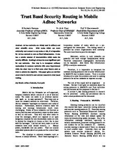
4.2.1 Limitations of OLSR in QoS Routing As mentioned, OLSR is a routing protocol for best-effort traffic, with emphasis on how to reduce the overhead, and at the same time, provide a minimum hop route. So in its MPR selection, the node selects the neighbor that covers the most unreached 2-hop neighbors as MPR. This strategy limits the number of MPRs in the network, ensures that the overhead is as low as possible. However, in QoS routing, by such an MPR selection mechanism, the “good quality” links may be “hidden” to other nodes in the network. As an example, we will consider the network topology in Section 4.1 again (see Figure 2.) The numbers along the lines indicate the available bandwidth over the links. As explained
20
in Section 4.1, in the OLSR MPR selection algorithm, node B will select C as its MPR. So for all the other nodes, they only know that they can reach B via C. Obviously, when D is building its routing table, for destination B, it will select the route D-C-B, whose bottleneck bandwidth is 3, the worst among all the possible routes.
5 A
E 60
D 3 40
110
B
10
10
F
25
C 50
100
30
G
Figure 2: Bandwidth-QoS Network Example for MPR Selection
Also, when “bandwidth” is considered to be the QoS constraint, in building the routing tables, nodes can no longer use the “Shortest Hosp Path” algorithm as proposed in [12], as the path with the minimum hops may not be the path with best bandwidth. Because of these limitations of OLSR in QoS routing, we revise it in two aspects: MPR selection and routing table computation, which are described in the following two subsections separately.
4.2.2 Changing the MPR Selection Criteria The decision of how each node selects its MPRs is essential to determining the optimal bandwidth route in the network. In the MPR selection, a “good bandwidth” link should not be omitted. In other words, as many nodes as possible that have high bandwidth links connecting to the MPR selector must be included into the MPR sets. Based on this idea, three revised MPR selection algorithms are presented.
21
4.2.2.1 OLSR_R1 In the first algorithm, MPR selection is almost the same as that of the original OLSR described in Section 4.1. However, when there is more than one 1-hop neighbor covering the same number of uncovered 2-hop neighbors, the one with the largest bandwidth link to the current node is selected as MPR: 1. start with an empty MPR set 2. select as MPRs those nodes in N which provide the “only path” to some nodes in 2-hop neighbors N2 3. while there exist nodes in N2 which are not covered { select as an MPR a 1-hop neighbor which reaches the maximum number of uncovered nodes in N2. If there is a tie, the one with higher bandwidth is chosen. } 4. As an optimization, process each node y in MPR. If MPR\(y) still covers all nodes in N2, y should be removed from the MPR set. The network in Figure 2 would select MPRs for node B as follows, based on OLSR_R1: Nodes B
1 hop Neighbors A, C, F, G
2 hop Neighbors D, E
MPR(s) F
Table 2: MPR Selected in OLSR_R1
Between C and F, F is selected as B’s MPR because it has the larger bandwidth.
4.2.2.2 OLSR_R2 The idea behind OLSR_R2 is to select the highest bandwidth neighbors as MPRs: 1. start with an empty MPR set 2. select as MPRs nodes in neighbors N which provide the “only path” to some nodes in 2-hop neighbors N2 22
3. while there exist nodes in N2 which are not covered { 3.1.Select as MPR a node that has the highest bandwidth link connected with the current node. If there is a tie, the one that covers more uncovered 2-hop neighbors is selected 3.2.Mark the neighbors of the newly selected MPR as covered in the 2-hop neighbor set of the current node } For example, using this algorithm, based on Figure 2, node B’s MPR(s) would be: Nodes B
1 hop Neighbors A, C, F, G
2 hop Neighbors D, E
MPR(s) A, F
Table 3: MPR Selected in OLSR_R2
Among node B’s neighbors, A, C, and F have a connection to its 2-hop neighbors. Among them, link BA has the largest bandwidth. So A is first selected as B’s MPR, and the 2-hop neighbor D is covered. Similarly, F is selected as MPR next and E is covered, so all 2-hop neighbors are covered and the algorithm terminates.
4.2.2.3 OLSR_R3 The third algorithm selects the MPRs in a way such that all the 2-hop neighbors have the optimal bandwidth path through the MPRs to the current node. Here, optimal bandwidth path means the bottleneck bandwidth path is the largest among all the possible paths. 1. start with an empty MPR set 2. select as MPRs nodes in neighbor N which provide the “only path” to some nodes in 2-hop neighbors N2 3. while there exist nodes in N2 which are not covered
23
{ 3.1.select as MPR a node so that the current node has the optimal route through the MPR to a 2-hop node 3.2.mark the 2-hop node as covered } Look again at node B in Figure 2 as an example. In order to cover D, neighbors A, C, or F need to be chosen as an MPR. Bandwidths available from B to D for three different routes are: B –110- A –5- D
bottleneck bandwidth is 5
B –50- C –3- D
bottleneck bandwidth is 3
B –100- F –10- D
bottleneck bandwidth is 10
The algorithm chooses the route with the largest bottleneck (in 2 hops). In this case the chosen MPR is F. In the same way, C is chosen as MPR by B to cover E. Nodes B
1 hop Neighbors A, C, F, G
2 hop Neighbors D, E
MPR(s) F, C
Table 4: MPR Selected in OLSR_R3
The three revised OLSR MPR selection algorithms may improve the chance that a better bandwidth route is found. However, by using such algorithms, the overhead may also increase compared with the original OLSR algorithm because we may increase the number of MPRs in the network, especially for OLSR_R3, which may select a different MPR for each 2-hop neighbor. In the simulations done in the static network model and the mobile Ad-Hoc network model, we analyze these algorithms to determine what kind of improvement we obtain and what price (in terms of the additional overhead) we have to pay for the achievement.
24
4.2.3 Routing Table Calculation Besides the MPR selection method, a node also needs to change the “Shortest Hops Path” algorithm in its routing table computation to reflect the bandwidth as the QoS metric. Here, two algorithms are introduced. One is the “maximum bandwidth spanning tree” proposed by us; the other is the extension of Bellman-Ford shortest path algorithm presented by [9]. The following sub-sections discuss the two algorithms separately.
4.2.3.1 Maximum Bandwidth Spanning Tree Algorithm Similar to the ordinary definition of a “minimum spanning tree”, the definition of the “maximum bandwidth spanning tree” is: using the bandwidth over the link between two nodes as weight, a maximum bandwidth spanning tree is a tree connecting all the nodes in the network whose total weight is maximal among all the possible trees. Theorem 1: The optimal bandwidth-constrained path from source to destination is along the maximum bandwidth spanning tree edge. Proof (by contradiction): Suppose there is a maximum bandwidth spanning tree T. Assume that the route from s to d in T is s->b->g->e->d, and in that route, there is a link l connecting b and g, which is the bottleneck bandwidth link of the route. Assume that there is another route from s to d, whose bottleneck bandwidth is greater than the route in T. Without loss of generality, we assume that there is a better route: s->c->e->d, and the link l’ connecting c and e is not in T, see Figure 3a.2
2
We can safely assume that l’ is not in T: otherwise, there would be two paths from s to d, which would violate the basic premise that we are dealing with trees. Also, the assumption that only l’ is not in T is correct: If the better route contains several links that are not in T, we can easily substitute them with the edges in T because T reaches each node in the graph.
25
Figure 3: Graphs to Prove Maximum Spanning Tree Algorithm
Furthermore, since l’ is a link on a better route, its weight has to exceed the weight of the bottleneck link l: weight(l’)>weight(l). Consider the tree T. When we remove l from T, T is divided into two separate graphs, G’ and G”, where s is in G’. T is originally a spanning tree, there is only one route from s to d in T through l. So after removing l, s and d are no longer connected, then s and d must
26
be in different parts. As s is in G’, d is in G”, see Figure 3b. When we add l’ to (b), the result is graph G, see Figure 3c. 1. We first show that G is still a spanning tree: s and d are in two separate graphs, s and d are not connected. As defined before, s and d can be connected through l’, which means when we add l’ to G’ and G”, the two separate graphs, G’ and G”, are connected together by l’. 1) From the way we construct G, we can see that all the nodes that are originally connected by T are now connected by G. 2) G’ and G” are originally part of spanning tree T, so G’ and G” are acyclic. l’ connects the originally separated G’ and G”, G’+G”+l’ is acyclic, so G is acyclic. 2. Based on the above, G is a spanning tree, whose weight is total weight of the original tree – weight(l) + weight (l’) > total weight of the original tree. However, according to the definition of the maximum bandwidth spanning tree, the total weight of such a tree is the largest among all the trees. So our above assumption is contrary to the definition, which means the optimal bottleneck bandwidth path is on the maximum bandwidth spanning tree edge. This completes the proof. Therefore, by building the “maximum bandwidth spanning tree”, the node can find the optimal path in its known partial network topology. Same as ordinary “minimum spanning tree” algorithm, the computational complexity of the “maximum bandwidth spanning tree” is O (E logV), where V is the number of nodes in the network, E is the number of links between the nodes. In Section 5.2, we will prove that each node indeed has enough partial topology information to correctly construct this graph.
27
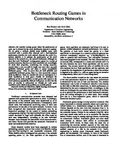
4.2.3.2 Extended BF Algorithm [9] describes an algorithm which computes the best bandwidth paths from a source to any reachable destinations with minimum hop count (shortest-widest path). This algorithm is based on a Bellman-Ford (BF) shortest path algorithm. The BF algorithm has a property that, at its hth iteration, it identifies the optimal cost path between the source and each destination, among paths of at most h hops. In the “Extended BF” algorithm, the cost is the bottleneck bandwidth along the path. In detail, at the kth iteration of the algorithm, the maximum bottleneck bandwidth to all destinations on a path of no more than k hops is recorded together with the corresponding routing information. When the algorithm terminates, the maximum bottleneck bandwidth paths with the smallest number of hops are found. Figure 4 is the pseudocode for the shortest-widest path algorithm form [9]. According to [9], the computational complexity of this algorithm is O (E logV), where V is the number of nodes in the network, E the number of links between them. So the “Extended BF” algorithm has the same complexity as the “Maximum Bandwidth Spanning Tree” algorithm.
28
Input: V = set of vertices, labeled by integers 1 to N. L = set of edges, labeled by ordered pairs (n,m) of vertex labels. s = source vertex (at which the algorithm is executed). For all edges (n,m) in L: * b(n,m) = available bandwidth on the edge between vertices n and m. H = maximum hop-count (at most the graph diameter). Variables: TT[1..N, 1..H]: topology table, whose (n,h) entry is a tab_entry record, such that: TT[n,h].bw is the maximum available bandwidth (as known thus far) on a path of at most h hops between vertices s and n, TT[n,h].neighbor is the first hop on that path (a neighbor of s). It is either a router or the destination n. S_prev: list of vertices that changed a bw value in the TT table in the previous iteration. S_new: list of vertices that changed a bw value (in the TT table etc.) in the current iteration. The Algorithm: begin; for n:=1 to N do /* initialization */ begin; TT[n,0].bw := 0; TT[n,0].neighbor := null TT[n,1].bw := 0; TT[n,1].neighbor := null end; TT[s,0].bw := infinity; reset S_prev; for all neighbors n of s do begin; TT[n,1].bw := b[s,n]); TT[n,1].neighbor := n; S_prev := S_prev union {n} end; for h:=2 to H do /* consider all possible number of hops */ begin; reset S_new; for all vertices m in V do begin; TT[m,h].bw := TT[m,h-1].bw; TT[m,h].neighbor := TT[m,h-1].neighbor end; for all vertices n in S_prev do begin; for all edges (n,m) in L do if min( TT[n,h-1].bw, b[n,m]) > TT[m,h].bw then begin; TT[m,h].bw := min( TT[n,h-1].bw, b[n,m]); TT[m,h].neighbor := TT[n,h-1].neighbor; S_new := S_new union {m} end end; S_prev := S_new; if S_prev=null then h=H+1 /* if no changes then exit */ end; end.
Figure 4: Pseudocode for Extended BF Algorithm
29
Both the “maximum bandwidth spanning tree” algorithm and the “extended BF” algorithm guarantee that the maximum bottleneck bandwidth path is found. However, the “extended BF” algorithm also guarantees that the path with the minimum hop counts among the best bandwidth paths is selected, while the “maximum bandwidth spanning tree” algorithm may compute a path with larger hop count. So in the simulations, we will use the “extended BF” algorithm for the routing table computation.
30
Chapter 5
QoS OLSR Evaluation in Static Networks In this chapter, we give the simulation result based on the static network case and prove that two of our heuristics proposed in Chapter 4 are indeed optimal, i.e., guarantee that the bandwidth-optimal path is found.
5.1. Static Network Simulation Result In this section, we simulate our MPR selection algorithms and compare the results. In the simulations done in this chapter, we assume that the Ad-Hoc network topology is stable at one moment so that we can study the QoS routing problem on that stable graph. Actually, there are various circumstances where Ad-Hoc networks are rather stable: A wireless network consisting of Desktops, Laptops and printers for home business may keep its original topology for a long time until someone moves one of the Laptops to another room, for example. In next chapter, however, we will test our algorithms in a simulated mobile Ad-Hoc network environment to see what the impact of nodes movement and link-state updating have on the network performance. With bandwidth constraint as QoS metric, as decided in Section 3.3, it is reasonable to view the “bandwidth” as available bandwidth. Most probably, the devices in the Ad-Hoc network will be configured with the same wireless card, which means that all nodes in the network have the same maximum bandwidth. So we are only interested in how much of
31
the remaining bandwidth is available for new traffic.
However, in real networks,
bandwidth computation is a complex issue. Many papers such as [15] discuss how to compute bandwidth in Ad-Hoc networks. Here, we use a rather simple and straightforward approach: measuring how much time a node monitors an idle channel and thus is available to transmit new messages over a link (node’s idle time), which is similar to [1]. MAC protocols such as IEEE 802.11 are based on a carrier-sense capability of each node. We exploit this capability to determine, locally at each node, for what percentage of time the medium has been busy in the recent past. A busy medium may indicate that a neighbor is transmitting data over the shared wireless channel. However, it may also indicate that nodes even further away, but still within interference range, are using the media. A node can only successfully transmit during times when neither its immediate neighbors nor other nodes in its interference range are transmitting. This characterization of the available bandwidth is superior to and with lower overhead than proposals where nodes communicate with their immediate neighbors to exchange information about their committed bandwidth, ignoring nodes further away. The “available bandwidth” over a link connecting nodes A and B is proportional to the minimum of A’s idle time and B’s idle time, since both nodes have to be available for a successful transmission. Since the number of nodes and the traffic between them in each node’s interference range is different, the idle times of two adjacent nodes may well be substantially different. However, due to the shared nature of the wireless medium, it is always the case that the link bandwidth between two adjacent nodes A and B is always equal to or better than the bandwidth over any 2-hop connection between A and B (i.e., via some intermediate node C), as will be explained in more detail in Section 5.2.
32
Depending on the underlying MAC protocol, a node may not be able to use the whole idle time. In IEEE 802.11 networks, for example, a node will wait for a random backoff time after it detects that the link is idle. However, as such backoff times are deliberately kept short, we neglect them in the remainder of this thesis. Because of the unstable nature of Ad-Hoc networks, it is also important to decide how the idle time, which reflects the network traffic condition, should be maintained and updated. This issue will be addressed in the next chapter. In this chapter, we are dealing with “network snapshots”, evaluating the route selection heuristics in OLSR. Using a simulator written in C++, we randomly generate network topologies, and perform the computations on these fixed graphs, which represent snapshots of the AdHoc network state. As mentioned above, for the time being, we are currently not investigating how our algorithm should propagate and adapt to changes in topology or available bandwidth. The following are the simulation details:
5.1.1 Network Scenario •
Network area: 1000 M x 1000 M
•
Number of nodes: 100
•
Transmission range: 100 M, 200 M, 300 M
•
Bandwidth: Based on the analysis in this section, the available link bandwidth is computed as follows: Each node is randomly assigned an “idle time” ranging from 0 to 1. The available link bandwidth between two nodes is equal to the minimum of their idle time × maximum bandwidth. Here, we consider that in the Ad-Hoc network, each link has the same maximum bandwidth, 2 Mbps. For example, if node a’s idle time is 0.5 and node b’s idle time is 0.3, then the available
33
bandwidth over link ab is: 0.3 × 2Mbps = 600 kbps. These randomly generated “idle times” reflect the traffic condition in the network snapshot because the consumed bandwidth over each link reflects the traffic flows over that link.
5.1.2 Simulation Objective We implemented a total of 5 algorithms and applied them to the randomly generated network snapshots: 1) OLSR (Section 4.1) with “shortest hops path” route computation algorithm 2) OLSR_R1 (Section 4.2.2.1) 3) OLSR_R2 (Section 4.2.2.2) 4) OLSR_R3 (Section 4.2.2.3) (The above 2)-4) are all using the “Extended BF” algorithm for route computation) 5) Pure link state algorithm: each node floods its link state information into the entire network. Then, the best bandwidth routes are computed with the “Extended BF” algorithm. By doing this, the path with maximum bottleneck bandwidth is guaranteed to be found. Routes found by algorithms 1) through 4) are compared with the route found by algorithm 5), using the simulation model and metrics discussed below.
5.1.3 Simulation Model For each transmission range (100m, 200m, 300m), 100 network snapshots are generated. For each connected pair in the network, we run the 5 algorithms mentioned in Section 5.1.2 to find a route between each pair of nodes in the network. Results obtained show how often the route found by the first 4 algorithms (original OLSR, OLSR_R1, OLSR_R2, and OLSR_R3) has lower bandwidth than the route found by a pure link state 34
algorithm. If we cannot find the optimal path using the first 4 algorithms, we will present how sub-optimal the result is. Also, we characterize and compare the overhead of these 5 algorithms.
5.1.4 Simulation Results Results are given in two categories: performance and cost. To further analyze the results, we also collect information about specific network characteristics.
5.1.4.1
Performance
Performance is characterized by "Error Rate" and “Average Difference”: •
“Error Rate” represents the percentage of times the standard OLSR, OLSR_R1, OLSR_R2, and OLSR_R3 algorithms do not find the optimal bandwidth path. In other words, Error Rate = total number of bad routes in 100 snapshots computed by OLSR / total number of optimum routes in 100 snapshots.
•
“Average Difference” is the average of the difference between the optimal bandwidth and current bandwidth found in routing algorithms in percentage: result = average of (bandwidth on optimal path-bandwidth on route computed)/bandwidth on optimal path, when the optimum routes are not found. The larger the value is, the worse the result.
5.1.4.2
Cost
The cost of the protocol is measured by “overhead” and “MPR percentage”: •
“Overhead”: How many control messages (messages originated by the nodes indicating who select it as MPR) are transmitted/re-transmitted in the network.
35
Overhead = the average number of control messages transmitted per snapshot/100 (the number of nodes in network). •
“MPR Number”: Average number of MPRs in the network. The more MPRs in the network, the higher the overhead.
5.1.4.3
Network Characteristics
We collect the average number of 1-hop neighbors and 2-hop neighbors for a node. These values affect the MPR number in the network. On one hand, the more 1-hop neighbors a node has, the less MPRs it may select, because with a high probability a small subset of its 1-hop neighbor can reach a high number of the 2-hop neighbors (assuming high connectivity of the network). On the other hand, the more 2-hop neighbors a node has, the more MPRs may be needed to cover them all.
5.1.4.4
Simulation Results and Analysis
Simulation Results are presented in Table 5 and Table 6. Transmission range 1-hop neighbors 2-hop neighbors
300M 21 33
200M 10 15
100M 2 4
Table 5: Network Characteristics
•
First we consider the results of all 5 algorithms for the same network, using the 300 M transmission range network as example (see Table 6): Considering the performance of the 4 OLSR algorithms, we see that the original OLSR has the worst performance – it has the highest “Error Rate” and “Average Difference”, which means in the 300 M transmission range network, the original OLSR has the highest probability that it can not find the best bandwidth path. At the same time, the bandwidth difference between the paths it finds and that of the
36
optimal path is also large. Although the OLSR_R1 uses the same MPR selection algorithm as the original OLSR, it achieves a large improvement in performance, which shows lower “Error Rate” and lower “Average Difference”. Such improvement is affected by the “Extended BF” algorithm, which finds the optimal path on the partial network a node learns from the procedure of MPR selector declaration and retransmission. However, OLSR_R1 does not always find an optimal path, as its MPR selection algorithm may omit the optimal bandwidth link from the partial network topology the node learned. (See the example of Section 4.2.1). However, OLSR_R2 and OLSR_R3 show very good results – each time, these two algorithms find the optimal bandwidth route. The explanation for this extremely good result is given in Section 5.2. Algorithm
Original OLSR OLSR_R1
OLSR_R2
OLSR_R3 Pure Link State Algorithm
Transmission Range 300 M 200 M 100 M 300 M 200 M 100 M 300 M 200 M 100 M 300 M 200 M 100 M 300 M 200 M 100 M
Performance Error Rate Average Difference 28% 41% 12% 14% 21% 8% 0% 0% 0% 0% 0% 0% 0% 0% 0%
46% 51% 45% 22% 26% 44% 0% 0% 0% 0% 0% 0% 0% 0% 0%
Overhead
Cost MPR Number
12 24 5 12 24 5 18 33 5.7 26 38 5.7 1245 979 28
65 68 42 65 68 42 70 72 45 71 73 44 100 100 100
Table 6: Summary of Simulation Results
As mentioned earlier, costs are directly related to the number of MPRs selected by the algorithms. The higher the number of MPRs in the network is, the higher the overhead. This relationship is clearly shown in the “Cost” category.
37
Of the 5
algorithms, in its MPR selection, standard OLSR emphasizes on reducing the number of MPRs in the network to lower the overhead. so it has the lowest MPR number and overhead compared with OLSR_R2, OLSR_R3 and Pure Link State Algorithm. (OLSR_R1 has almost the same MPR selection mechanism as that of standard OLSR, and these two algorithms therefore have comparable overheads.) Also, as predicted in Section 4.2.2, OLSR_R2 and OLSR_R3 select more MPRs, thus produce higher overhead than standard OLSR. Compared with OLSR_R2, OLSR_R3’s overhead is even higher, which is also consistent with our prediction. For Pure Link State algorithm, it obviously has the highest overhead, with each node acting as MPR, retransmitting the messages it receives. The result of all 5 algorithms in networks with a transmission range of 200 M and 100 M network have similar characteristic as the 300 M transmission range case. •
We also explored the performance of the individual algorithms: Standard OLSR: At first glance, it may seem strange that a network with a node transmission range of 200 M has the highest overhead. Intuitively, the denser the network is, the higher the overhead: for the same number of nodes and area size, the network contains more edges if the transmission range of a node is higher (see Table 5). However, the result can be explained as follows: in general, the more MPRs are selected, the higher the overhead. In a higher density network (such as for a node transmission range of 300 M), node connectivity is also high, so a node may need fewer MPRs to cover its 2-hop neighbors. On the contrary, in lower density network (such as for a node transmission range of 100 M), because of the lower connectivity, a node may have fewer 2-hop neighbors; therefore, it also needs fewer MPRs.
38
However, the transmission range of 200 M falls within these two extremes, so it may well result in the largest number of MPRs to produce the highest overhead. This situation is not found in the Pure Link State Algorithm, where a node’s entire neighbor set is its MPR set. So the denser the network is, the more neighbors/MPRs a node has, resulting in a higher overhead. Also, one may expect that the denser the network is, the worse the performance should be. With higher connectivity, there are more possible routes from a given source to a destination, and the probability that OLSR chooses a non-optimal route is higher. This tendency can be seen when comparing the performance of 300 M and 100 M transmission range networks. But again the 200 M transmission range network is the exception, having the highest “Error Rate”. Considering a node in an optimal bandwidth route, its next hop node on the path is its 1-hop neighbor, and the hop after next is its 2-hop neighbor (proof is given in Section 5.2). In other words, an optimal bandwidth path is composed of segments “node->1-hop neighbor -> 2-hop neighbor”. The route computed by OLSR has that feature as well. For 100 M transmission range, because of its lower connectivity, the node has less 1-hop neigbhors and 2-hop neighbors. As a result, in this network, there are fewer segments of “node->1-hop neighbor -> 2-hop neighbor”, resulting in a lower propability that OLSR chooses the wrong path. For the dense network (300 M transmission range), a node has many more 1-hop and 2-hop neighbors, resulting in many segments of “node->1-hop neighbor -> 2-hop neighbor”. The selected MPRs will cover many of the 2-hop neighbours more than once, again resulting in a lower propability for OLSR ignoring the segments belonging to the optimal path. As shown by the difference between
39
OLSR and OLSR_R1, a simple change in how to calculate the paths, based on the same MPR set, can yield significant performance improvements. Again, the 200 M transmission range case falls between these two extremes, resulting in the worst performance. OLSR_R1: the result shows the same trends as that of the original OLSR. Also, when comparing the performance of the original OLSR and OLSR_R1, it shows that OLSR_R1 achieves larger improvements over the original OLSR in higher density network. That is because for higher density networks, more links are declared to a node. So when computing its routing table, a node has more choices in path selection. The original OLSR uses the Shortest Hops Path Algorithm for route computation, which is unsuitable for bandwidth QoS routing. So the probability that the original OLSR picks up a non-optimal path is higher in denser networks. OLSR_R2 and OLSR_R3: Regarding performance, they both find the optimal path. Regarding the cost, they also exhibit the phenomenon that a 200 M transmission range network has the highest MPR number/overhead. The reason is the same as the one explained above for standard OLSR. Pure Link State Algorithm: Comparing the original OLSR with the Pure Link State Algorithm, we find that the higher the network density, the more obvious the overhead reduction is achieved by the original OLSR. This is consistent with the declaration in [12] that the denser the network is, the more optimization OLSR will achieve, compared to the Link State Algorithm.
40
5.2. Correctness of the Revised OLSR Algorithm From the simulation results, we find that under the current simulation model, both OLSR_R2 and OLSR_R3 always find the optimal path. Can these two algorithms guarantee the optimal result? This is indeed the case. Following is the proof: Theorem 2: OLSR_R2 finds the optimal bandwidth path. LEMMA 1: The intermediate nodes on one of the optimal paths (the path with the highest bottleneck bandwidth) are all selected as MPRs by the previous nodes on the path. Proof: A node in the route may not be selected as the MPR by the previous node if: 1) the node does not provide connection to that node’s 2-hop neighbors and 2) the node does not meet the MPR selection criteria. In the following proof, we address these two situations separately. 1) A direct link between two nodes a and b always has same or better available bandwidth than any routes connecting a and b via some intermediate nodes. Proof: In the following graph, there are two paths from a to b: link (ab) and link (a, n1, n2, n3,…nk, b). b a
nk
n1 n2 n3 Figure 5: Two Different Paths Connect Node a and Node b
Suppose node a, b, n1, n2, n3,…nk’s idle time are Ia, In1, In2, In3, Ink, Ib respectively. As discussed in section 5.1.1, the wireless medium studied here is the shared channel. A node can only successfully transmit during times no nodes in its interference range
41
are transmitting (the channel is idle), and as both the two nodes a and b on the link ab should be available during the transmission, which means that the bandwidth over link ab should be min(Ia, Ib). And also, we suppose here that all the nodes in the network are configured with same data rate. So based on the concave nature of the available bandwidth, bandwidth of link (AB) and link (A, N1, N2, N3,…Nk, B) are •
Link (ab): min(Ia, Ib)
•
Link(a, n1, n2, n3,...nk, b) : min of bandwidth on links(AN1, N1N2, N2N3, ...NkB) = min (Ia, In1, In2, In3,...Ink, Ib)
It is clear that link (AB) provides the same or better bandwidth path because min(Ia, Ib)≥min(Ia, In1, In2, In3,...Ink, Ib) � The direct path connecting two nodes has the same or better available bandwidth than the path via any intermediate nodes. Also, we can conclude that if a node has no connection to its neighbors’ 2-hop neighbors, it is not on the optimal path, as this is the path via the intermediate node (the 1-hop neighbor that connects to another 1-hop neighbor). 2) There is an optimal path from source to destination such that all the intermediate nodes on the path are selected as MPR by their previous nodes on the same path. Proof:
Without loss of generality, we suppose that in an optimal path, S, M1,
M2…Mk, Mk+1,…Mr, D, there are nodes in the route which are not selected as MPRs by their previous nodes. Also, based on the result of 1), we can assume that for each node on the path, its next node on the path is its 1-hop neighbor, and the node two hops away from it is its 2-hop neighbor. For example, M1 is S’s 1-hop neighbor, M2 is
42
S’s 2-hop neighbor. Mk+1 is Mk’s 1-hop neighbor, Mk+2 is Mk’s 2-hop neighbor, etc (see Figure 6).
S
D R1
M1
M2
Rk Mk
Mk+1
Mk+2
Mp
Mq
Mr
Figure 6: Route from Source S to Destination D
a) Suppose that on the optimal route, the first intermediate node M1 is not selected as MPR by source S. However, M2 is the 2-hop neighbor of S. Based on the basic idea of MPR selection that all the 2-hop neighbors of a node should be covered by this node’s MPR set, S must have another neighbor R1, which is selected as its MPR, and is connected to M2. According to the criteria of MPR selection specified in OLSR_R2, S selects R1 instead of M1 as its MPR because the link bandwidth of SR1 is better than the link bandwidth of SM1, which means Ir1 (idle time of node R1) is larger than or equal to Im1 (idle time of node M1). Define bottleneck bandwidth of route R as B(R). B(S->R1->M2->…->Mr->D) = min(B(S->R1->M2), B( M2->…->D)) = min(min(Is, Ir1, Im2), B(M2->…->D)) B(S->M1-> M2->…->D) = min(min(Is, Im1, Im2),B( M2->…->D))
43
As Ir1 ≥ Im1, min(Is, Ir1, Im2) ≥ min(Is, Im1, Im2) � B(S->R1->M2->…->Mr->D) ≥ B(S->M1->…->D). Based on our assumption, route S->M1-> M2->…->D is optimal path � S->R1-> M2->…->D is also an optimal path � Source’s MPR are on the optimal path. b) Assume that on the optimal route S->M1->…->Mk->…->D, all the nodes on segment M1->Mk are selected as MPR by their previous node, we now prove that the next hop node of Mk on the optimal route is Mk’s MPR. Suppose that Mk+1 is not Mk’s MPR. Same as above, Mk+2 is the 2-hop neighbor of Mk, so Mk must has another neighbor Rk, which is the MPR of Mk and has connection to Mk+2. Again, Mk selects Rk instead of Mk+1 as its MPR because link bandwidth MkRk is better than MkMk+1, which means Irk (idle time of node Rk) is better than Imk+1 (idle time of node Mk+1). B(S->...Mk->Mk+1->Mk+2->…Mr->D) = min(B(S->Mk), min(Imk, Imk+1, Imk+2), B( Mk+2->D)) B(S->…Mk->Rk->Mk+2…->D) = min(B(S->Mk), min(Imk, Irk, Imk+2), B( Mk+2->D)) ≥ B(S->...Mk->Mk+1->Mk+2->…Mr->D) As S->…->Mk->MK+1->Mk+2->…->D is optimal route � S->…->Mk->Rk->Mk+2…->D is also optimal route. � In an optimal route, the (k+1)th intermediate node is the MPR of the (k)th intermediate node.
44
Based on a) and b), all the intermediate nodes of an optimal path are the MPRs of the previous nodes. LEMMA 2: A node can correctly compute the optimal path for the whole network topology. Proof: 1) as shown by Section 4.2.3.1 and 4.2.3.2, using a “Maximum Bandwidth Spanning Tree Algorithm” or “Extended BF Algorithm”, a node can compute the optimal path on the known partial network topology 2) In OLSR, each node knows the links between MPRs and their selectors in the network. Based on LEMMA 1, there is an optimal path such that all the intermediate nodes on it are the MPR of the previous node on the same path. So the optimal path for the whole network topology is included in the partial topology the node knows. � The node can correctly compute the optimal path for the whole network topology.
Theorem 3: OLSR_R3 finds the optimal bandwidth path. The proof is similar to that of Theorem 2.
45
Chapter 6
OPNET Simulation Environment Chapter 5 compared the performance of original OLSR protocol and the QoS OLSR versions in the static network case. In this and the following chapters, simulations for the OLSR algorithms are done in OPNET to show the algorithms’ performance with node movements and data flows.
6.1
Introduction to OPNET
Originally developed at MIT, OPNET [18] is a network simulator allowing researchers to design and study communication networks, devices, protocols, and applications. An OPNET simulation package includes three main graphic editors – network editor, node editor, and process editor. The network editor manages network topologies; the node editor controls network devices’ performance; the process editor implements protocols, resources, applications, algorithms, and queuing policies. These three editors work together to provide various simulation environments. In OPNET, the Wireless LAN protocol is based on the IEEE 802.11 carrier sense multiple access and collision avoidance (CSMA/CA) distributed coordination function (DCF) access scheme. The unicast data packets are transmitted with the RTS/CTS frame exchange to reserve media, and the “Data and Acknowledgement” frame exchange to ensure the transmission reliability. The broadcast data packets, however, can be
46
transmitted after sensing an idle channel, but may suffer from the collision by the hiddenterminal problem. In the simulation, modifications are done to the OPNET Wireless LAN model to calculate the available bandwidth, which will be discussed in the following Section 6.2.
6.2
OLSR Simulation in OPNET
6.2.1 The Original OPNET OLSR Model The original OLSR model in OPNET was developed by the Naval Research Laboratory (NRL) of the United States. Figure 7 is an OLSR node in OPNET Node Editor.
Figure 7: OLSR Node
47
In the above OLSR node model, except for the “olsr” process model and the “udp_gen” process model (see the box in upper part of Figure 7), all the other process models are the standard process models of OPNET. •
“olsr” process model
The “olsr” process model implements the OLSR routing protocol discussed in Section 4.1. The following Figure 8 shows the OLSR implementation in the OPNET Process Model. After initialization and sending an empty Hello message to begin the process, the OLSR routing protocol continuously goes to “itimer” state to decide if it is time to send a Hello message or a TC message. If yes, the message is sent and olsr returns to “idle” state. When a packet (Hello message or TC message) arrives, it goes to “proc_msg” state, processes the received message, and updates the routing table, if necessary.
Figure 8: OLSR Process Model
48
•
“udp_gen” process model
Figure 9 is the “udp_gen” process model. It generates “udp” packets, which serve as the application data packets in simulations. At the same time, it records how many “udp” packets are received at the current node, providing a mechanism to evaluate the packet delivery ratio of a routing protocol.
Figure 9: UDP_GEN Process Model
6.2.2 QoS OLSR OPNET Model Based on the discussion in Section 4.2, the following revisions are made to develop the QoS OLSR node model: 1) Idle time calculation3 As mentioned before, QoS OLSR uses the media idle time to reflect the available bandwidth over a link. This task is done by modifying the standard OPNET Wireless LAN model.
3
In the real word, the wireless card keeps on monitoring the wireless physical medium before it sends packets, same as the implementation of the transmitter and the receiver in OPNET Wireless LAN model. So, the information we use to calculate idle time in OPNET could also be obtained somehow through the interface of the wireless card.
49
Each OLSR node connects to the wireless media (see the box in lower part of Figure 7). The OPNET Wireless LAN simulation model is composed of a wireless_lan_mac process model
(wireless_lan_mac),
a
transmitter
(wlan_port_tx_0_0),
a
receiver
(wlan_port_rx_0_0), and channel streams (the dotted line between the wireless_lan_mac and the transmitter or receiver). If the node is sending packets, its transmitter becomes busy. If there are other nodes beginning transmission within the interference range of the current node, its receiver senses the busy media and sends a media busy signal. As the OPNET Wireless LAN model already defines functionalities to capture changes of the media, the media idle time is computed as following: In a 0.5 second time period4, we record how long the transmitter or receiver is busy (time between the transmitter or receiver becomes busy and then returns to idle again). Then the percentage of idle time is calculated, which is (0.5-busy time)/0.5. This is a sample of the idle time in this interval. We calculate the idle time of 10 such 0.5-second-periods in a row, obtain 10 samples of idle time over 5 seconds, arrange these samples into a sliding window, and calculate its average value. When an 11th idle time sample is obtained, the 1st idle time in the sliding window is deleted, and the 11th idle time is inserted into the sliding window as the last value. See the following Figure 10 as an example: The Wireless LAN process model continuously calculates idle time, and reports the average value to the OLSR process model.
4
As in OLSR, Hello message is sent every 0.5 second, we use 0.5 second as the sampling period to reflect the traffic condition in the wireless media.
50
position
0
1
2
3
4
5
6
7
8
9
Idle time
50%
50%
50%
50%
50%
50%
50%
50%
50%
50%
Original average idle time is 50%. After new value is obtained, the updated sliding window:
the 11th value (30%) is obtained
position
0
1
2
3
4
5
6
7
8
9
Idle time
50%
50%
50%
50%
50%
50%
50%
50%
50%
30%
New average value: (50% x 9 + 30%)/10=48% Figure 10: Example of How Idle Time Is Calculated
2) Idle time propagation As discussed in Section 4.2.2 and Section 4.2.3, the QoS OLSR versions needs to know the available bandwidth on the neighbor link to select MPRs, and the available bandwidth of the far away link to compute the routing table. As idle time should be used to calculate the available bandwidth on the links, we revise the format of OLSR Hello and TC messages to include the idle time in it. 5 a. Hello message: in addition to the original information such as neighbor address and neighbor link type, a node also includes its own idle time in the Hello messages. Upon receiving a Hello message from its neighbor, a node reads the neighbor idle time, and selects MPRs using the QoS MPR selection algorithm.
5
For compatibility, it is better to introduce a new message type to propagate idle time together with the original OLSR message. However, for simplicity, for the time being, we simply revise the original OLSR message.
51
b. TC message: the TC message originator not only puts its own idle time in TC messages, but also piggybacks its MPR selectors’ idle times, which are obtained from the Hello messages. When a node receives TC messages, it knows the idle time information of both the TC message originator and the MPR selectors, thus gets information about the links and the link bandwidth between the TC message originator and its MPR selectors. In this way, it learns the partial network topology and the bandwidth condition of that partial network, and is ready to calculate the routing table. Also, QoS OLSR needs to decide when to originate a TC message. In the original OLSR, if a node detects changes in its MPR selector, it generates a new TC message to propagate the changes in the network topology. In QoS OLSR, however, changes in link bandwidth condition must also be propagated for the correct computation of the best bandwidth routes. However, because of the dynamic nature of the Ad-Hoc network, link bandwidth may change all the time. If an MPR generates a TC message as soon as it detects a bandwidth change over the link between its MPR selector and itself, there will be too many messages flooding into the network, causing extremely high overhead. So in our QoS OLSR, some “threshold” of bandwidth change is defined. If an MPR finds there is “significant bandwidth change”, that is, the available bandwidth raises or drops a certain percentage, between the links of its MPR selectors and itself, it will generate a new TC message informing the whole network about the change, enabling other nodes to update their routing table reflecting such changes. There is a tradeoff in how to define the “threshold”. On one hand, if the “threshold” is low, TC messages will be generated as soon as there is a small percentage change of the bandwidth. That will cause frequent generation of TC messages, introducing high overhead, although more accurate
52
bandwidth information is obtained. On the other hand, if the “threshold” is high, TC messages will not be generated until there is a very large percentage change of the bandwidth. Thus, the overhead is reduced, but the nodes only obtain relatively inaccurate bandwidth information. In the implementation, a node keeps on informing its original idle time in its Hello messages until the latest idle time value it obtains from the Wireless LAN process model changes above the “threshold” compared with the original idle time. In such case, the node will propagate the new idle time in the Hello message, reflecting the change in the traffic condition on the wireless media. Upon receiving such Hello message, the neighbor node re-selects MPRs according to the latest idle time information. Consequently, TC messages are generated to reflect the bandwidth change. In the simulation, we will define different “threshold” values to compare the network performance, and analyze the “price” paid and the “profit” gained. 3) MPR selection Based on the simulation result of the static network case in Chapter 5, we find that OLSR_R2 (Section 4.2.2.2) guarantees to find the best bandwidth path while it has a lower overhead compared with OLSR_R3 (Section 4.2.2.3), which also finds the optimal bandwidth path. So in the implementation of QoS OLSR model, we use OLSR_R2 as the MPR selection mechanism. 4) Routing table calculation As discussed in Section 4.2.3, the “Extended BF” algorithm is used to compute the routing table, as it not only finds the best bandwidth path, but the shortest path as well.
53
5) Idle time recording In order to observe the routing protocols in bandwidth QoS aspect, the network bandwidth condition as well as the network topology should be recorded. As OPNET does not provide such information, a data-recording process model is developed, which takes network snapshot as the simulation goes on. Every 5 seconds6, the data-recoding model records the positions of all nodes in the network, their idle times computed by the modified Wireless LAN model, which is discussed in 1), and the actual routing table each node computed. Using such information, the optimal bandwidth paths in the network snapshot can be computed, and the bandwidth difference between the routes the routing algorithms calculated and the optimal routes can be obtained.
6.3
Simulation Setup
The following environments are defined for OPNET simulations: Movement Space: 1000m x 1000m flat space Number of Nodes: 50 nodes, 30 nodes7 Simulation Time: 900 seconds. Many papers that study the performance of routing protocols in Ad-Hoc network such as [22] use 900 seconds as simulation length. Besides, after 30 seconds of simulation time, the routing algorithms’ performance such as packet delivery ratio and delay is rather stable. So we decide to also use 900 seconds simulation time for all scenarios.
6
It is desirable to use even shorter time interval to obtain more accurate network information. However, because of disk space limitations, a 5 seconds interval is used here. Compared with OPNET’s 9 seconds interval for exporting simulation result, 5 seconds seems to be a reasonable choice. 7 The simulation results for a dense network (50-node-network) are presented in Chapter 7; the simulation results for a sparse network (30-node-network) are presented in Chapter 8.
54
Movement Model: each node randomly selects a destination in the 1000m x 1000m area, moves to that destination at a speed distributed uniformly between 0 and “maximum speed”. After it reaches the destination, the node selects another destination and another speed between 0 and “maximum speed”, and moves again. The model is based on the “random waypoint” model [13], but differs from the “random waypoint” model in that in “random waypoint” model, the node pauses for “pause time” seconds before it moves again, while in current movement model, nodes move continuously. In the simulation, there are 5 “maximum speed” values: 20m/s, 10m/s, 5m/s, 1m/s, and 0m/s. Communication Model: packet sources are the udp_gen process models defined in the OLSR node model. In each simulation, there are 20 communication pairs. Each source sends 64-byte packets at a rate of 4 packets/second. So in total, 80 packets are sent each second. OPNET Model Parameter: see Table 7. Hello Interval 0.5s TC Interval 2s Data Rate 2 Mbps Buffer Size 256000 bits Wireless LAN Parameters Retry Limit 7 Wireless LAN 250 M Propagation Range OLSR Parameters
Table 7: OPNET Model Parameter
Routing Protocol: 4 routing protocols – Original OLSR, QoS OLSR with 20% bandwidth updating threshold (20% OLSR), QoS OLSR with 40% bandwidth updating threshold (40% OLSR), and QoS OLSR with 80% bandwidth updating threshold (80% OLSR). All the QoS OLSR algorithms use the OLSR_R2 mechanism to select MPRs, and the “Extended BF” algorithm to calculate the routing table.
55
For each of the 5 movement patterns (maximum speed 20m/s, 10m/s, 5m/s, 1m/s, 0m/s), 3 simulations are done for each routing protocol to test its performance. The 3 simulations differs from one another in 1) nodes starting positions, 2) communication pairs, 3) the random destinations and the uniformly distributed speed a node chooses in its movement.
56
Chapter 7
Simulation in OPNET – Dense Network In this section, simulation results on dense network (50-nodes-network) are presented and analyzed. The results are grouped into two sets: Basic Performance and QoS Performance. 1) Basic Performance – the basic performance is the set of metrics used by most routing protocols for result comparison: “Packet Delivery Ratio” and “End to End Delay”. •
Packet Delivery Ratio: percentage of packets that successfully reach the receiver nodes each second. Packet Delivery Ratio = average packet received per second / 80 (the total packet sent per second) * 100%
•
End to End Delay: the average time between a packet being sent and being received
2) QoS performance – the metrics that relate to the bandwidth QoS routing studied in this paper: “Error Rate” and “Bandwidth Difference”. •
Error Rate: the percentage of times the routing algorithms do not find the optimal bandwidth path.
•
Bandwidth Difference: the average difference between the optimal bandwidth and current bandwidth in percentage, which is less than the optimal one, found in routing algorithms. Result = average of (bandwidth on optimal path - bandwidth on route computed)/bandwidth on optimal path, when the optimum routes are not found.
57
For all simulation results presented in this and the next chapter, two kinds of data are shown: one is the average result, which is listed in the upper part of the table cell; the other is the width of the confidence interval, calculated with 95% confidence, which is in the lower part of the table cell.
7.1
Basic Performance
Table 8 shows the Basic Performance results of the 4 OLSR routing algorithms (QoS 20%, QoS 40%, QoS 80%, original) for 5 movement patterns (maximum speed: 20m/s, 10m/s, 5m/s, 1m/s, 0m/s). (Here, PK Delivery Ratio=Packet Delivery Ratio; E-to-E Delay=End to End Delay)
Speed: 20m/s
QoS 20% QoS 40% QoS 80% Original
Speed: 10m/s
E-to-E Delay (ms)
PK Delivery Ratio
E-to-E Delay (ms)
PK Delivery Ratio
E-to-E Delay (ms)
66.89% 2.96% 67.59% 1.39% 72.05% 5.20% 75.75% 2.91%
24.92 2.64 20.16 2.83 24.70 23.54 8.58 3.16
75.71% 0.63% 79.21% 4.63% 79.91% 4.30% 82.30% 3.28%
14.82 2.31 13.70 7.19 18.88 17.33 5.73 0.64
84.66% 1.74% 88.05% 2.68% 89.46% 3.95% 87.81% 1.20%
9.55 1.11 10.43 1.89 7.78 4.93 5.28 1.54
Speed: 1m/s
QoS 20% QoS 40% QoS 80% Original
Speed: 5m/s
PK Delivery Ratio
Speed: 0m/s
PK Delivery Ratio
E-to-E Delay (ms)
PK Delivery Ratio
E-to-E Delay (ms)
90.89% 2.28% 94.31% 2.14% 93.44% 7.28% 96.34% 0.49%
9.20 4.98 9.84 5.16 7.09 6.72 4.67 1.13
98.15% 3.16% 99.53% 0.48% 97.58% 6.90% 98.54% 1.00%
13.05 8.16 9.04 7.09 8.11 5.77 5.88 2.52
Table 8: Packet Delivery Ratio and End-to-End Delay Comparison for 50-Node-Network Scenario
58
7.1.1 Packet Delivery Ratio Figure 11 shows the comparison of the packet delivery ratio the 4 algorithms achieve under different movement patterns. Packet Delivery Ratio 106.00% 101.00% 96.00% QoS 20%
91.00%
QoS 40%
86.00%
QoS 80%
81.00%
Original
76.00% 71.00% 66.00%
20m/s
10m/s
5m/s
1m/s
0m/s
QoS 20% 66.89% 75.71% 84.66% 90.89% 98.15% QoS 40% 67.59% 79.21% 88.05% 94.31% 99.53% QoS 80% 72.05% 79.91% 89.46% 93.44% 97.58% Original
75.75% 82.30% 87.81% 96.34% 98.54%
Figure 11: Comparison of Packet Delivery Ratio for 4 OLSR Algorithms in 50-Nodes-Network
From high movement (maximum speed 20m/s) to low movement (maximum speed 0m/s), packet delivery ratio for all algorithms rises continuously. It is easy to understand. With the lower movement, the established links between the nodes have a lower probability to break, thus, there are less stale routes in the node routing tables, which results in a higher ratio for correct packet delivery. However, in the 4 OLSR algorithms, the original OLSR outperforms the other 3 QoS version of OLSR algorithms in packet
59
delivery, especially at high mobility (maximum speed: 20m/s). There are two reasons behind it: a. High Overhead: As mentioned in Chapter 4, the original OLSR protocol concentrates on how to reduce the overhead, and tries to minimize the MPR sets to reduce the TC messages flooding into the network. However, the QoS versions of OLSR attempt to select the best bandwidth path, so in their MPR selection mechanism, they select neighbors with high idle time as MPR, resulting in a larger MPR set than the original OLSR protocol. So more TC messages are generated and relayed into the network by QoS OLSR versions. The following Table 9 and Figure 12 and 13 show the average TC messages generated or relayed by all MPRs in the network (in packets and in kbps) for the 4 algorithms:
Figure 12: TC Packet Sent in Packet/S
60
Figure 13: TC Packet Sent in Kbps
TC Sent
QoS 20% QoS 40% QoS 80% Original
Speed: 20m/s
Speed: 10m/s
Speed: 5m/s
Speed: 1m/s
Packets/s
Kbps
Packets/s
Kbps
Packets/s
Kbps
Packets/s
Kbps
816.00 16.38 726.74 29.36 614.09 48.42 439.15 19.19
600.99 31.64 501.94 18.04 423.48 32.44 156.77 11.53
755.62 45.86 630.68 18.52 497.39 54.88 372.13 57.29
543.67 24.49 442.19 23.03 339.89 8.27 128.55 19.23
649.36 51.02 558.60 15.30 424.62 59.14 305.48 14.11
458.36 55.41 379.11 21.75 289.51 29.35 102.45 8.04
510.88 110.21 423.28 122.43 306.99 90.25 200.51 75.23
341.16 71.65 279.17 67.55 205.76 48.53 64.78 21.68
TC Sent QoS 20% QoS 40% QoS 80% Original
Speed: 0m/s Packets/s
Kbps
406.71 57.64 362.46 17.74 347.48 30.66 236.66 102.56
232.14 55.68 214.85 24.74 209.53 33.04 69.62 28.81
Table 9: Comparison of TC Message Sent for 4 OLSR Algorithms in 50-Node-Network Scenario
From the table and the figures, we can see that for all algorithms, there are fewer TC messages sent at lower movement than at higher movement. This is because at lower movement, less TC messages are generated to reflect topology changes. Also, 20% OLSR has the highest number of TC messages generated and relayed, while the original OLSR protocol has the least number of TC messages. Under the same speed, the
61
difference of TC messages sent between the original OLSR protocol and the 3 QoS OLSR versions comes from three aspects: 1) The original OLSR protocol only generates TC messages to reflect topology change, while QoS OLSR versions also need to generate TC messages to reflect bandwidth change; with a lower bandwidth update threshold, more TC messages are generated to reflect bandwidth change, causing the highest overhead in 20% OLSR 2) The average TC packet length in QoS OLSR versions is larger then that of the original OLSR protocol, as in the QoS OLSR versions, TC messages not only include the addresses of the MPR selectors, but also their idle times. 3) QoS OLSR versions have larger MPR sets than the original OLSR protocol, so more TC messages are generated and relayed by the larger MPR sets. Among the QoS OLSR algorithms, 20% OLSR may select more MPRs than 40% and 80% OLSR. The following is the explanation: As mentioned in Section 6.2.2, in QoS OLSR, a node continues announcing its original value of idle time in the Hello messages until its own idle time rises or drops over a certain threshold; then, the node announces its new idle time. Also, nodes select MPRs based on the link bandwidth, in other word, neighbors’ idle time. Based on the way the idle time is calculated, at the beginning of the simulation, the whole wireless media is idle, so all nodes’ initial idle times are 100%. With a low idle time updating threshold such as 20%, the neighbor idle times are more diverse than with high idle time updating thresholds such as 40% or 80%. Recall that if the neighbor idle times are the same, a node selects the one that covers most un-reached 2-hop-neighbors as MPR. Otherwise, it keeps on selecting neighbors with higher idle
62
time as MPRs until all the 2-hop-neighbors are covered. So a neighbor set with more diversity of idle times may result in a higher number of MPRs, see Figure 14 as an example.
Figure 14: MPR Selection in QoS OLSR with Different Thresholds
From Figure 14, we can see that if a node’s neighbor set has a high diversity of idle time values, the node may have a higher probability to select more MPRs, depending on the network topology. With the possibly larger MPR set, more TC messages are generated and relayed by 20% OLSR than 40% OLSR and 80% OLSR.
63
The overhead (TC messages sent) in the fixed network differs a little from the above observation. The overhead for 20% and 40% OLSR still keeps the same trend as before – the number of TC messages sent in the fixed network is less than for a maximum speed of 1m/s. However, more TC messages are sent in 80% OLSR and the original OLSR for movement 0m/s than 1m/s. The explanation is that in the fixed network, where there is no node movement, in the original OLSR, TC messages are sent regularly at 2s interval. So the TC message overhead is solely related to the number of MPRs in the network, which depends on the network topology. The network topology does not change during the simulation, and we only run 3 simulations for each algorithm under each movement pattern. For the fixed network case, actually, we just take 3 samples of network “snapshots”, which may not be enough to give an exact result. The 80% OLSR may have the same problem in the fixed network, as with a large threshold for bandwidth updates, TC messages sent in the network may mainly be decided by the number of MPRs in the network, which does not change often in the static network. Considering the confidence interval, there is a large overlap for the value shown for 1m/s and 0m/s scenario, which means there is not too much overhead difference between the extremely low movement scenario (1m/s) and the no movement scenario (0m/s), which is consistent with our basic explanation. With higher overhead introduced into the network, especially for the 20% OLSR at higher movement, the wireless media is extremely busy, imposing a negative impact on the packet delivery rate for QoS versions of OLSR.
64
b. Incorrect Routing Table: besides the delay of topology updating information, which causes stale routes in the routing table, the following Figure 15 shows another typical scenario that causes incorrect topology information:
Figure 15: An Example for TC Packet Collisions at the Physical Layer
In Figure 15, based on the original OLSR algorithm, node_2 is selected as MPR by node_1, and generates a TC message advertising that there is a link between node_1 and node_2. Node_3 and node_4 are all MPRs of node_2, so they both relay the TC message. Suppose at that time, the wireless media is idle, node_3 and node_4 relay that TC message immediately, most probably at the same time. As a result, the TC messages collide at node_6, and node_6 does not know that it can reach node_1 through node_2. From this example, we can see that if there are overlapped two hop neighbors covered by
65
multiple MPRs, there is a high probability that TC packets collide at these neighbors, causing problems in routing table calculation. This problem happens in all 4 OLSR algorithms. But because of the different MPR selection mechanism, the QoS OLSR algorithms have more overlapped two hop neighbors than the original OLSR protocol, causing more TC message collisions. How does the above two reasons impact on the packet delivery ratio of the Ad-Hoc routing protocol? Table 10 shows the breakdown of unsuccessfully delivered packets. In Table 10, besides the information about “TC sent”, the following metrics are also presented: •
Packet Un-delivered: the average number of udp data packets that do not reach the destination in each second. Packet Un-delivered=(1-Packet Delivery Ratio)*80, as total packets sent by the network in each second is 80
•
IP PK Dropped: average number of packets dropped at the IP layer each second. This is an OPNET build-in metric, which represents the number of packets dropped at the IP layer because there is no entry about the destination in the IP routing table. (The IP routing table does not know the next hop for a certain destination.)
•
Control Bad PK:
the average number of TC or Hello packets that experience
collision at the wireless_lan_mac layer each second. This is an important metric to reflect the correctness of the routing table built by the routing algorithm. As TC messages include information about the network topology, the collision of TC messages means that the node could not get the updated topology information abut the remote part of the network, and could not correctly build the routing table, which will result in packet dropping in either the IP layer (the remote node is reachable, but
66
the routing table does not include such entry) or the Wireless LAN layer (a packet is sent to a node out of the transmission range based on a stale route in the routing table. As the sending node cannot receive the Ack, it keeps on retransmission until the retry limit is passed and the packet is dropped.) •
Data Bad PK: the average udp data packets that experience collision at the wireless media in one second. A data packet experiencing collision doesn’t necessarily mean it can not be correctly delivered, as a data packet can be re-transmitted for 7 times before it is dropped.
•
WLAN PK Dropped: average number of packets dropped at the wireless_lan_mac layer. This is also an OPNET build-in metric. There are two reasons for packets dropped in this layer: 1) the overflow of higher layer buffer, and 2) failure of all retransmissions until retry limit (7). Both reasons are related to the control overhead/TC messages sent —on one hand, if there are many control packets, the wireless media is very busy, the probability that the data packet experiences collision is high, and the probability that it is dropped because of all retry chances are used up is also high; on the other hand, too many packets waiting to be processed also causes the overflow of the higher layer queue.
67
Speed
20m/s
10m/s
5m/s
1m/s
0m/s
Algorithm
TC Sent
Packet
IP PK
Control
Data
WLAN PK
(pks/s)
Un-delivered
Dropped
Bad PK
Bad PK
Dropped
(pks/s)
(pks/s)
(pks/s)
(pks/s)
(pks/s)
QoS 20%
816.00
26.49
6.15
2481.03
29.65
20.23
OLSR
16.38
2.37
2.40
235.82
2.69
1.50
QoS 40%
726.74
25.93
4.12
2064.78
25.32
21.82
OLSR
29.36
2.83
0.93
86.87
3.99
0.64
QoS 80%
614.09
22.36
1.84
1767.88
17.22
20.39
OLSR
48.42
4.16
0.38
100.65
4.29
4.17
Original
439.15
19.40
0.64
1285.95
11.39
18.67
OLSR
19.19
2.33
0.33
120.24
0.87
2.38
QoS 20%
755.62
19.43
5.24
2252.42
28.54
14.12
OLSR
45.86
2.31
0.72
82.66
0.68
1.21
QoS 40%
630.68
16.63
3.32
1891.44
20.79
13.26
OLSR
18.52
3.70
2.35
135.10
7.10
1.38
QoS 80%
497.39
16.07
1.82
1454.60
17.35
14.18
OLSR
54.88
3.44
0.79
112.75
3.37
3.75
Original
372.13
14.16
2.09
1087.10
9.85
12.00
OLSR
57.29
2.62
1.09
117.35
3.49
1.51
QoS 20%
649.36
12.27
4.30
1920.89
27.34
7.93
OLSR
51.02
1.39
0.65
249.25
2.87
0.73
QoS 40%
558.60
9.56
2.03
1605.54
19.30
7.50
OLSR
15.30
2.14
1.35
116.99
7.75
1.07
QoS 80%
424.62
8.43
1.60
1248.21
12.94
7.47
OLSR
59.14
3.16
1.57
51.94
3.04
3.80
Original
305.48
9.75
0.62
818.62
11.67
9.11
OLSR
14.11
0.96
0.72
153.38
1.07
0.53
QoS 20%
510.88
7.29
4.96
1435.72
33.57
2.32
OLSR
110.21
1.82
0.49
188.93
20.67
1.28
QoS 40%
423.28
4.55
2.13
1172.97
20.87
2.40
OLSR
122.43
1.71
0.56
198.05
19.26
1.50
QoS 80%
306.99
5.25
3.01
1129.49
13.43
2.22
OLSR
90.25
5.82
5.28
189.08
15.11
1.54
Original
200.51
2.93
0.75
476.91
9.87
2.17
OLSR
75.23
0.39
1.39
100.98
5.41
1.01
QoS 20% OLSR
406.71 57.64
1.48 2.53
1.37 2.53
829.73 178.96
33.35 17.15
0.10 0.04
QoS 40% OLSR
362.46 17.74
0.38 0.38
0.36 0.36
731.52 89.79
21.34 23.99
0.01 0
QoS 80% OLSR
347.48 30.66
1.94 5.52
1.93 5.49
718.25 113.65
19.60 28.92
0 0
Original OLSR
236.66 102.56
1.17 0.80
1.16 5.06
355.19 212.67
13.07 7.06
0 0
Table 10: Where Are the Unsuccessfully Delivered Packets Dropped?
68
Let us take the 20m/s scenario as an example. Referring to Figure 16, we can see that because the original OLSR protocol has the smallest MPR set, it has the smallest number of control packet collisions (see the category of “Control Bad PK), resulting in the smallest number of packets dropped at the IP layer (“IP PK Dropped”). Also, it has the smallest number of packets dropped at the Wireless LAN (“WLAN PK Dropped”). Compared with the QoS OLSR versions, its low overhead results in a relatively less busy wireless media, reducing the possibility of overflow of higher layer queue and packet collisions.
Figure 16: Relationship between Packets Undelivered and Packets Dropped at Different Layers (20m/s)
Among the 3 QoS OLSR algorithms, as discussed before, 20% OLSR may have the largest MPR set, because with the more accurate link bandwidth information, it may select more MPRs than the other two QoS algorithms, resulting in more overlapped two hop neighbors. This is why the 20% OLSR has the largest number of TC message collisions, and the largest number of packets dropped at the IP layer. With the same
69
reason, the 80% OLSR gets the most correct information about the network topology and has the lowest number of packets dropped at the IP layer. The packets dropped in the Wireless LAN of the 3 QoS OLSR algorithms, however, are very close, although the 20% OLSR introduces much more control traffic into the network. To explain this phenomenon, recall that the route computation of QoS OLSR always directs data traffic to the routes with higher bottleneck bandwidth, which means, ideally, the data traffic in the 20% OLSR always chooses a route that is less busy, causing relatively low overflow compared with its high overhead level. The behavior of the 4 OLSR algorithms in other movement patterns can be analyzed similarly. Note that at lower speed scenarios (5m/s, 1m/s, and 0m/s), the packet delivery ratio for the QoS OLSR versions is close to the original OLSR protocol. At low movement, the control overhead is reduced for all algorithms, resulting in a relatively less busy wireless media. Consequently, the additional overhead introduced by QoS OLSR versions will not have as negative an effect on the packet delivery as in high movement scenarios. From the data collected, we can also concluded that the main reason for the packet delivery ratio difference among the 4 OLSR algorithms is the correctness of routing tables calculated, as the difference in the “IP PK Dropped” among all 4 algorithms is almost the same as the difference in “Packet Un-delivered”.
7.1.2 End-to-End Delay Based on Table 7, Figure 17 shows the End-to-End Delay for each algorithm under each movement pattern.
70
Packet End to End Delay (ms) 30.00 25.00 20.00
QoS 20% QoS 40%
15.00
QoS 80% Original
10.00 5.00 0.00
20m/s
10m/s
5m/s
1m/s
0m/s
QoS 20%
24.92
14.82
9.55
9.20
13.05
QoS 40%
20.16
13.70
10.43
9.84
9.04
QoS 80%
24.70
18.88
7.78
7.09
8.11
Original
8.58
5.73
5.28
4.67
5.88
Figure 17: Comparison of End-To-End Delay of Data Packets for 4 OLSR Algorithms in 50-NodesNetwork
Basically, for all movement patterns, the original OLSR has the lowest delay. It is easy to understand. As the original OLSR has the lowest overhead, its network is the least congested, resulting in the least delay. Also, the original OLSR algorithm always computes the shortest hop path, while the QoS OLSR versions may compute longer paths because they target on the best bottleneck bandwidth path, which also affects the end-toend delay of the data packets. For the three QoS OLSR algorithms, we can see that at higher movement speed (20m/s and 10m/s), the 80% threshold QoS OLSR has a higher delay, while at lower movement speed (5m/s, 1m/s and 0m/s), its delay is close to the original OLSR. To analyze this phenomenon, recall that the 80% threshold QoS OLSR has the most inaccurate 71
bandwidth information of the network, which means that the routing algorithm may select a route that is still relatively congested. At higher movement, all the QoS OLSR algorithms have higher overhead because of the frequent updates due to topology change (see Table 9 and Figures 12, 13), making the network congested. Working on the already congested networks, 20% QoS OLSR and 40% QoS OLSR do a better job in directing the traffic to the less congested routes, resulting in the lower packet delay. However, at lower movement speed, there are much less topology updates, so the more frequently sent bandwidth update messages in 20% and 40% OLSR tend to make the network busy, resulting in a larger delay than the 80% OLSR. Again, for all algorithms, the delay is reduced with speed dropping from 20m/s to 1m/s, with the exception for a speed of 0m/s. The packet delay in static networks is higher than the delay in networks with 1m/s movement. In the static and low movement network, because of the low control overhead, packet delay may mainly be affected by the length of the path the packet travels. In the static network, because there is no movement, there is a higher probability that the communication pairs are far away, which does not change in the simulation time. In the 1m/s scenario, nodes change positions, resulting on average in a shorter path length than in the static network. That is why the delay in the 1m/s network is lower than that in the static network.
7.2
QoS Performance
In this sub-section, the QoS performance of the 4 OLSR routing algorithms is discussed. Figure 18, 19, and Table 11 show the “Average Difference” and “Error Rate” among the 4 algorithms under different movement patterns.
72
Speed
20m/s
10m/s
5m/s
1m/s
0m/s
Algorithm QoS 20% OLSR QoS 40% OLSR QoS 80% OLSR Original OLSR QoS 20% OLSR QoS 40% OLSR QoS 80% OLSR Original OLSR QoS 20% OLSR QoS 40% OLSR QoS 80% OLSR Original OLSR QoS 20% OLSR QoS 40% OLSR QoS 80% OLSR Original OLSR QoS 20% OLSR QoS 40% OLSR QoS 80% OLSR Original OLSR
Bandwidth Difference 10.17% 1.53% 15.41% 0.98% 25.80% 2.07% 28.96% 0.60% 9.89% 0.52% 15.57% 1.18% 25.57% 0.18% 30.97% 2.86% 9.41% 0.78% 14.26% 1.64% 25.63% 0.80% 30.33% 2.45% 9.19% 1.80% 14.61% 0.82% 21.12% 3.13% 27.51% 1.09% 8.98% 0.58% 13.18% 3.07% 18.99% 2.74% 19.54% 5.17%
Error Rate 18.19% 0.41% 26.71% 4.98% 37.17% 2.77% 43.29% 2.22% 17.50% 0.62% 26.35% 2.42% 39.65% 3.41% 43.55% 0.38% 18.25% 0.83% 26.69% 1.92% 38.70% 3.60% 46.35% 2.28% 18.76% 2.33% 28.98% 4.43% 40.64% 3.13% 47.68% 3.20% 13.37% 9.60% 26.24% 23.40% 43.65% 14.34% 53.28% 16.17%
Table 11: QoS Performance Comparison of 4 OLSR Algorithms in 50-Nodes-Network
73
Average Bandwidth Difference 35.00% 30.00% 25.00%
QoS 20%
20.00%
QoS 40%
15.00%
QoS 80% Original
10.00% 5.00% 0.00% 20m/s
10m/s
5m/s
1m/s
0m/s
Figure 18: Comparison of Average Bandwidth Difference for 4 OLSR Algorithms in 50-NodesNetwork
Error Rate 60.00% 50.00% 40.00%
QoS 20% QoS 40%
30.00%
QoS 80%
20.00%
Original
10.00% 0.00% 20m/s 10m/s 5m/s 1m/s 0m/s
Figure 19: Percentage of Time the 4 OLSR Algorithms Do Not Find the Optimal Bandwidth Route in 50-Nodes-Network
74
All QoS OLSR outperform the original OLSR in both the “Error Rate” and “Bandwidth Difference”. Among the QoS OLSR algorithms, 20% OLSR updates the bandwidth condition most frequently, introducing the highest overhead, but gets the most accurate bandwidth information. So the routes it calculates are closest to the optimal routes. The 40% and 80% OLSR, however, update bandwidth information less frequently, introducing less overhead, but their QoS performances are not as good as that of 20% OLSR. In the above, the results for “Bandwidth Difference” and “Error Rate” of each algorithm are calculated based on its own network conditions – the bandwidth difference between the routes the routing algorithm calculated and the optimal paths in the network in which the routing algorithm works are presented. However, because the QoS OLSR versions introduce more overhead than the original OLSR protocol, the networks in which the QoS OLSR versions work may have worse overall available bandwidth than that of the original OLSR algorithm. So one may question if the QoS OLSR versions really improve the route bandwidth condition. To clarify, the average available bandwidth over the routes the routing algorithms computed is presented as follows: (Please note, as in our model, available bandwidth = maximum bandwidth x idle time in percentage, here, the available bandwidth is shown as percentage of idle time.) To calculate the average available bandwidth on the routes the routing algorithms calculate, first, we obtain the average optimal routes bandwidth, see Table 12.
75
Algorithm QoS 20% OLSR QoS 40% OLSR QoS 80% OLSR Original OLSR
20m/s 77.68% 4.18% 82.23% 7.20% 78.17% 18.16% 87.07% 5.37%
10m/s 80.93% 6.12% 84.92% 1.60% 84.27% 5.20% 87.28% 3.00%
5m/s 82.29% 4.92% 86.29% 2.45% 87.17% 1.26% 90.63% 4.03%
1m/s 84.69% 3.55% 87.46% 1.53% 90.08% 2.54% 91.14% 1.72%
0m/s 89.73% 0.46% 90.17% 0.97% 92.34% 2.48% 93.08% 0.43%
Table 12: Available Bandwidth on the Optimal Paths in the Network the Routing Algorithm Works (Measured as Idle Time)
The above results are consistent with our former analysis: The lower the moment speed, the less the overhead all the OLSR algorithms introduce into the network. So from speed 20m/s to 0m/s, the optimal bandwidth conditions for all the OLSR algorithms rise continuously. The original OLSR algorithm has the least overhead, so the network where it works always has the best bandwidth condition. Compared with 80% OLSR, 40% OLSR evenly directs traffic throughout the network, so under high movement (speed 20m/s, and 10m/s) where the wireless media are rather busy, 40% OLSR has better optimal bandwidth routes than that of the 80% OLSR, although it has more overhead than 80% OLSR. Under low movement (speed 5m/s, 1m/s, and 0m/s), the added overhead of 40% OLSR has a negative effect on the network bandwidth condition, thus the 40% OLSR has less optimal bandwidth than 80% OLSR. As the 20% OLSR has the highest overhead, its optimal bandwidth routes have the lowest available bandwidth. Then, we calculate the actual average available bandwidths on the routes the routing algorithms compute. The actual average available bandwidth the routing algorithms calculated = the available bandwidth on the optimal paths x ((1- “Bandwidth Difference”) x “Error Rate”) + (1- “Error Rate”))
76
= the available bandwidth on the optimal paths x (1- “Bandwidth Difference” x “Error Rate”) Using the “Bandwidth Difference” and “Error Rate” values in Table 11, the result for actual average available bandwidth the routing algorithms calculated is shown in Figure 208.
Figure 20: Average Available Bandwidth (in Idle Time) on the Routes the 4 OLSR Algorithms Compute (50-Nodes-Network)
8
As the calculation includes multiply operation, we do not calculate the width of the confidence interval for the “actual average bandwidth the routing algorithms calculated”.
77
From the above, we can see that although the QoS OLSR introduces more overhead into the network, the rout it computes still have better available bandwidth than the original OLSR. In movement patterns with maximum speed 20m/s, 10m/s, 5m/s, and 1m/s, among all the OLSR algorithms, the 40% OLSR always computes the route with the best available bandwidth, as it has less overhead than 20% OLSR and more accurate bandwidth information than 80% OLSR. In the fixed network case, because of few topology updates, all the algorithms have low overhead. Thus, 20% OLSR find the routes with highest bandwidth, for it has the most accurate bandwidth information. From the above results, we are convinced that the QoS OLSR versions do achieve bandwidth improvement over the original OLSR algorithm.
7.3
Analyzing Simulation Result with Confidence Interval
The above Section 7.1 and Section 7.2 analyze the simulation result based on the average value. In this section, we look at the confidence intervals to see which sets of the performance of the 4 OLSR algorithms are statistically significant and which are not. 1) Packet Delivery Ratio Figure 21 shows the comparison of the Packet Delivery Ratio for all the 4 OLSR algorithms under all movement patterns. In each graph, the value of the upper and lower end of the vertical line is the upper and lower bound of the Packet Delivery Ratio of each OLSR algorithm; the points which are connected by the line crossing the graph are the average values. If there is no overlap of the range of the confidence interval, we can say that the algorithms’ difference in performances is statistically significant.
78
Figure 21: Packet Delivery Ratio Comparison with Confidence Intervals
79
From the graphs, we can see that in high movement patterns (20m/s and 10m/s), the observed Packet Delivery Ratio performance improvement of the original OLSR protocol over the 20% OLSR and 40% OLSR is statistically significant. However, with low movement patterns (5m/s, 1m/s, and 0m/s), the 4 algorithms’ difference in performance is not statistically different. This is consist with our analysis in Section 7.1.1 – with higher movement speed, the added overhead of 20% and 40% OLSR have a negative effect on the Packet Delivery Ratio, because the networks are already congested with frequently topology update message. 2) End-to-End Delay Figure 22 shows the End-to-End Delay with confidence intervals. All the values shown have the unit “ms”. In movement patterns 20m/s, 10m/s, and 5m/s, the confidence intervals for 20% OLSR and 40% OLSR have no overlap with the confidence interval for original OLSR, which means the difference of End-to-End Delay performance between 20% OLSR and 40% OLSR and the original OLSR is statistically significant. Although the range of the confidence interval of the End-to-End delay in 80% OLSR overlaps the original OLSR, its large interval means that the End-to-End Delay performance of 80% OLSR is highly variable. On the whole, because of the large overhead that the QoS OLSR algorithms introduce into the network, they result in a higher delay than the original OLSR. In the static networks (speed 0m/s), the End-to-End Delay performance of the 4 algorithms is rather close. Because of the low overhead in the static network, the delay may mainly be decided by the hop counts of the routes the 4 algorithms computed, which may not significantly differ from one another.
80
Figure 22: End-To-End Delay Comparison with Confidence Intervals
81
3) QoS Performance Figure 23 presents the QoS Performance comparison for all 4 OLSR algorithms with confidence interval.
Figure 23: QoS Performance Comparison with Confidence Intervals
From the graphs, we can see that for movement patterns 20m/s, 10m/s, 5m/s, and 1m/s, the 20% OLSR’s performance improvement over 40% OLSR, 40% OLSR’s over 80%
82
OLSR, and 80%’s over the original OLSR in QoS aspect is statistically significant. In the fixed network scenarios, the 4 OLSR algorithms’ confidence interval range overlap with one another, except that 20% OLSR’s performance improvement over the original OLSR in Bandwidth Difference and Error Rate is statistically significant. This is because in the fixed network, with few TC messages for topology update, the bandwidth conditions on the alternative routes do not significantly differ from each other.
7.4
Conclusions
Based on the simulation result presented and analyzed above, we can see that the QoS OLSR algorithms do enhance the network QoS performance. However, in order to achieve these improvements, additional “protocol overhead” is also introduced, which degrades the performance of these QoS routing protocols, especially with respect to “Packet Delivery Ratio” and “End-to-End Delay”. As there is a trade-off between the achievements the routing algorithms make and the price that is paid to get such achievement, the routing protocols should be selected carefully based on the request of the data application.
83
Chapter 8
Simulation in OPNET – Sparse Network In Chapter 7, OPNET simulation results in a dense network (50-nodes-network) are discussed. In the dense network, the QoS OLSR algorithms do improve the bandwidth condition on the routes computed, but with additional overhead, their basic performance is not as good as the original OLSR protocol, especially under high movement. In this chapter, simulations are done in a sparser network (30-nodes-network) to see if the situation is the same. The results are analyzed and compared with that of the 50-nodenetwork scenario. The network scenario for the simulations in the 30-nodes-network is almost same as that discussed in the Section 6.3, except that for 30-nodes-network, we do not run simulations on the fixed network (speed: 0m/s). As the network with 30 nodes is much sparser than the network with 50 nodes, there is a high probability that the 30-nodes-network is disconnected. Without node movement, the network performance such as packet delivery ratio is mostly decided by the node’s initial position, which we think is not interesting to study. So in the simulations, we only look at node movement patterns of maximum speed 20m/s, 10m/s, 5m/s and 1m/s. Similar to Chapter 6, the simulation results in the 30-nodes-network are presented in two sets: Basic Performance and QoS Performance.
84
8.1
Basic Performance
Table 13 summarizes the Basic Performance results of the 4 OLSR algorithms. Speed: 20m/s
QoS 20% QoS 40% QoS 80% Original
Speed: 10m/s
Speed: 5m/s
Speed: 1m/s
PK Delivery Ratio
E-to-E Delay (ms)
PK Delivery Ratio
E-to-E Delay (ms)
PK Delivery Ratio
E-to-E Delay (ms)
PK Delivery Ratio
E-to-E Delay (ms)
62.44% 5.11% 61.46% 7.90% 66.86 3.96 70.21% 8.43%
26.25 7.13 27.98 12.46 18.73 11.75 11.52 3.70
69.50% 9.30% 75.56% 5.11% 79.63% 5.46% 77.83% 2.91%
21.14 15.68 19.47 5.50 17.21 16.23 7.35 3.16
74.66% 1.70% 79.10% 10.09% 85.00% 5.79% 81.76% 8.09%
27.20 18.16 13.46 2.77 12.69 14.00 6.12 1.87
86.89 9.73 90.79 9.90 89.75 10.50 91.14 5.86
8.74 2.08 7.82 3.77 5.80 2.62 4.79 1.14
Table 13: Packet Delivery Ratio and End-to-End Delay Comparison for 30-Nodes-Network Scenario
8.1.1 Packet Delivery Ratio Figure 24 shows the comparison of average Packet Delivery Ratio of the 4 OLSR algorithms in 30-nodes-network. Same as the 50-nodes-network scenario, in the 30nodes-network, from high movement (speed 20m/s) to low movement (speed 1m/s), packet delivery ratio for all algorithms rises continuously. Also, in the 20m/s scenario, the original OLSR outperforms the QoS OLSR versions with respect to the Packet Delivery Ratio in the movement speed 10m/s and 5m/s, the 80% OLSR and the original OLSR protocol perform closely; in the extremely low movement pattern (1m/s), all the algorithms are close with respect to packet delivery ratio. The relationship of the average packet delivery ratio of the 4 OLSR algorithms in the 30nodes-network is similar to that of the 50-nodes-network. The reasons, of cause, are the same – the high overhead the QoS OLSR algorithms, especially the 20% OLSR introduced into the network cause more TC message collisions, and make the wireless media busier.
85
Packet Delivery Ratio 95.00% 90.00% 85.00%
QoS 20%
80.00%
QoS 40%
75.00%
QoS 80%
70.00%
Original
65.00% 60.00%
20m/s
10m/s
5m/s
1m/s
QoS 20%
62.44%
69.50%
74.66%
86.89%
QoS 40%
61.46%
75.56%
79.10%
90.79%
QoS 80%
66.86%
79.63%
85.00%
89.75%
Original
70.21%
77.83%
81.76%
91.14%
Figure 24: Comparison of Packet Delivery Ratio for 4 OLSR Algorithms in 30-Nodes-Network
However, when looking at the confidence interval of packet delivery ratio, we find that the width of the confidence interval for the 30-nodes-network is much larger than that of the 50-nodes-network. This is caused by the network partition – in a sparse network, nodes may not be all connected, and the Packet Delivery Ratio depends on the network topology, which may vary from one simulation to another. To see a clearer packetdelivery-performance comparison of the QoS OLSR versions and the original OLSR protocol with confidence interval, we introduce a metric called “Relative Packet Delivery Ratio”. The “Relative Packet Delivery Ratio” is the average difference of the Packet Delivery Ratio of the QoS OLSR versions with the original OLSR protocol in each simulation. If the value is positive, then on average, the QoS algorithm’s Packet Delivery Ratio is higher than the original OLSR protocol; if the confidence interval does not
86
crosses 0, then statistically speaking, the difference in Packet Delivery Ratio between the QoS OLSR and the original OLSR protocol is significant. Table 14 shows the “Relative Packet Delivery Ratio” of the 3 QoS OLSR algorithms compared with the original OLSR. Both the average value and the width of the confidence interval are presented. Algorithm QoS 20% OLSR QoS 40% OLSR QoS 80% OLSR
20m/s 10m/s -7.79% -8.33% 3.90% 6.53% -8.75% -2.26% 3.28% -2.24% -3.46% 1.81% 11.98% 2.65%
5m/s -0.71% 6.58% -2.66% 2.73% 3.24% 11.99%
1m/s -4.25% 4.05% -0.35% 4.04% -1.38% 4.64%
Table 14: Relative Packet Delivery Ratio of QoS Algorithms in 30-Nodes-Network
Figure 25 graphically shows the values in Table 14. Relative Packet Delivery Ratio (% ) 20.00 15.00 10.00 5.00 0.00 -5.00 -10.00 -15.00 -20.00
20m/s 20%
20m/s 40%
20m/s 80%
10m/s 20%
10m/s 40%
10m/s 80%
5m/s 20% 5m/s 40% 5m/s 80% 1m/s 20% 1m/s 40% 1m/s 80%
Figure 25: Relative Packet Delivery Ratio of QoS Algorithms in 30-Nodes-Network
Statistically, for speed of 20m/s and 10m/s, the 20% OLSR and 40% OLSR have less packets delivered than the original OLSR, while the performance of the 80% OLSR is almost the same as that of the original OLSR. For speeds of 5m/s and 1m/s, all QoS OLSR versions have similar Packet Delivery Ratio to the original OLSR protocol.
87
8.1.2 End-to-End Delay Figure 26 shows the End-to-End Delay of all OLSR algorithms.
Figure 26: End-To-End Delay Comparison for OLSR Algorithms in 30-Nodes-Network
Same as the 50-nodes-network scenario, on average, the original OLSR protocol, which has the lowest overhead, has the least End-to-End Delay for all movement patterns. For all algorithms, basically, delay is reduced when speed becomes lower, with the exception of 20% OLSR at speed 5m/s. However, considering the large width of confidence interval of the delay, we can conclude that the difference in the delay of 20% OLSR for movement patterns 20m/s, 10m/s and 5m/s is not statistically significant.
88
8.2
QoS Performance
Table 15 summarizes the QoS performance results for the 4 OLSR algorithms. Figure 27 and Figure 28 show graphically the QoS performance results. 20m/s 10m/s 5m/s 1m/s Bandwidth Bandwidth Bandwidth Bandwidth Algorithm Error Rate Error Rate Error Rate Error Rate Difference Difference Difference Difference 20% 12.71% 18.47% 13.63% 16.92% 13.89% 17.76% 10.82% 13.75% OLSR 1.37% 1.08% 5.16% 1.75% 0.07% 2.45% 1.98% 5.87% 40% 17.53% 22.63% 17.36% 21.57% 17.10% 20.40% 13.25% 19.29% OLSR 1.06% 0.67% 0.76% 1.66% 4.23% 2.94% 0.26% 1.90% 80% 21.45% 27.45% 23.13% 31.03% 23.24% 34.25% 17.92% 32.02% OLSR 2.20% 2.27% 3.27% 3.97% 0.97% 1.73% 7.85% 3.55% Original 26.44% 37.57% 24.35% 38.11% 23.94% 39.75% 20.15% 39.37% OLSR 1.07% 2.06% 2.04% 2.06% 4.67% 2.11% 3.27% 5.38% Table 15: QoS Performance Comparison for 4 OLSR Algorithms in 30-Nodes-Network
Figure 27: Comparison of Average Bandwidth Difference for 4 OLSR Algorithms in 30-NodesNetwork
89
Same as the 50-nodes-network, all QoS OLSR versions outperform the original OLSR protocol in both the “Error Rate” and “Bandwidth Difference”. Also, considering the confidence interval, the QoS OLSR algorithms’ QoS performance improvement over the original OLSR is statistically significant, especially in high speed movement scenarios (20m/s and 10m/s).
Figure 28: Error Rate Comparison in 30-Node-Network
Similar to Section 7.2, we obtain the available bandwidth on the optimal bandwidth routes of the networks in which the 4 OLSR algorithms work (see Table 16), and calculate the average available bandwidth on the routes the routing algorithms computed (see Figure 29). All the results are shown in terms of idle time.
90
Algorithm QoS 20% OLSR QoS 40% OLSR QoS 80% OLSR Original OLSR
20m/s 88.59% 1.95% 88.24% 2.47% 87.86% 4.92% 91.16% 1.40%
10m/s 89.76% 6.28% 88.41% 6.07% 90.49% 2.08% 91.73% 0.17%
5m/s 89.97% 11.15% 89.46% 11.09% 91.00% 8.57% 91.13% 8.57%
1m/s 89.39% 10.66% 88.22% 4.30% 86.24% 17.06% 92.60% 0.94%
Table 16: Available Bandwidth on the Optimal Paths in the Network the Routing Algorithms Works (30-Nodes-Network)
Figure 29: Average Available Bandwidth (in Idle Time) on the Routes the 4 OLSR Algorithms Compute (30-Nodes-Network)
Unlike the 50-nodes-network scenario where 40% OLSR computes the best available bandwidth routes, in 30-nodes-network case, the routes that 20% OLSR computes always have the best available bandwidth. In a sparse network, there is fewer control traffic in the network than in the dense network for all algorithms. So the additional overhead 20% OLSR introduces into the network does not have much negative effect on the network’s
91
bandwidth condition. With the most accurate bandwidth information, the 20% OLSR protocol computes the routes with highest bandwidth.
8.3
Comparison of the Results in 50-Nodes-Network and 30-
Nodes-Network From the discussion in Chapter 7 and Section 8.1, we can see that the simulation results of all OLSR algorithms in a dense network (50-nodes-network) and a sparse network (30nodes-network) have the following similarities: •
Basically, with the speed slowing down, all the algorithms have better Packet Delivery Ratio and End-to-End Delay in both a dense network and a sparse network.
•
The original OLSR protocol outperforms the QoS OLSR versions, especially 20% OLSR and 40% OLSR with respect to the basic performance metrics in high speed scenarios; while in the low speed scenarios, statistically speaking, their performance metrics are almost the same.
•
In all movement patterns, the QoS OLSR algorithms outperform the original OLSR protocol in “Bandwidth Difference” and “Error Rate”. Even considering the confidence interval, the QoS OLSR versions’ performance improvement in these two QoS aspects in high movement scenarios is statistically significant.
•
When considering the actual bandwidth condition the routes computed by the OLSR algorithms, the QoS OLSR version computes routes that have higher bandwidth than the routes of the original OLSR protocol.
Now, let us compare the difference of the simulation result between the dense network and the sparse network.
92
1) Packet Delivery Ratio From Figure 30, we can see that on average, the packet delivery ratio in the 50-nodesnetwork for all algorithms is better than that in the 30-nodes-network. Because of the network partition, some destinations in 30-nodes-network are temporarily un-reachable, causing lower packet delivery ratio in the 30-nodes-network.
Figure 30: Comparison of Packet Delivery Ratio in 50-Nodes-Network and 30-Nodes-Network
2) End-to-End Delay The average delay in the 30-nodes-network has a larger average value than that of the 50nodes-network (see Figure 31). It seems unreasonable, as with the lower control overhead in the sparse networks, one may expect that there is less delay. However, considering the large confidence interval in the delay results in 30-nodes-network, those results are not conclusive. With more simulations, we may get more accurate result, which is one of the items of future work.
93
Figure 31: Comparison of Delay in 50-Nodes-Network and 30-Nodes-Network
3) QoS Performance We compare the actual routes bandwidth the 4 OLSR algorithms compute in the dense and sparse networks. Referring to Figure 32, for all OLSR algorithms, the routes computed in the 30-nodes-network have higher bandwidth (in terms of idle time) than that in the 50-nodes-network. That is because in sparse networks, with fewer nodes generating control messages, the networks’ overall bandwidth conditions are better than that of the dense networks. In the 50-nodes-network, 40% OLSR computes the best bandwidth paths; in the 30nodes-network, 20% OLSR computes the best bandwidth paths. The reason also comes from the networks’ traffic load. As the overall network bandwidth condition is better in the sparse network than in the dense network, 20% OLSR, with the most accurate bandwidth information, computes the best bandwidth routes.
94
Figure 32: Routes Bandwidth Comparison in 50-Nodes-Network and 30-Nodes-Network
95
Chapter 9
Conclusion and Future Work In the thesis, we describe the importance of QoS routing in Ad-Hoc networks, the challenges we meet, and the approach we take. We discuss in detail our idea of adding support for QoS into the OLSR protocol, our three heuristics that allow OLSR to find the maximum bandwidth path, and show initial simulation results of these algorithms under a number of network snapshots. From a performance perspective, all three heuristic increase the odds of finding a path that is optimal under a bandwidth constraint. Also, we prove that for our Ad-Hoc model, two of the heuristics (OLSR_R2 and OLSR_R3) are indeed optimal. Besides analyzing the algorithms based on static network snapshots, we also add OLSR_R2 to an OLSR simulation based on OPNET to explore the impact of node movement and bandwidth change. In the simulations in OPNET, we not only compare the basic performance and the QoS performance of the original OLSR protocol and the QoS OLSR versions, but also analyze where their advantages and limits come from. As a result, we show that the QoS OLSR do improve the available bandwidth of the routes computed, but the added cost – the additional overhead also has a negative impact on the network in End-to-End Delay and Packet Delivery Ratio, especially in the high speed movement scenarios. As the added overhead is the main cost that affects the QoS routing algorithm’s performance, the future work on QoS routing in Ad-Hoc networks may be focused on how to reduce the overhead. The following are some basic ideas:
96
•
In the static network simulations, OLSR_R1 does not find the best bandwidth route all the time. However, it has much improvement over the original OLSR protocol, while has almost the same overhead as that of the original OLSR protocol. From the simulations in OPNET, we learned that the high overhead is the main reason for the inferior packet delivery ratio performance of the QoS OLSR versions, so it is interesting to implement OLSR_R1 in OPNET to observe its performance.
•
From the analysis of OPNET simulations, we see that the TC packet collisions at the 2-hop neighbors cause the problem of stale routing tables. TC message collisions happen when there are 2 MPRs relaying TC messages at the same time. This problem happens in both the original OLSR protocol and the QoS OLSR versions. To avoid this problem, we can add some jitter mechanism into OLSR protocol – when an MPR receives a TC message, it waits for a random delay time before it relays that TC message, instead of relaying it immediately. We could implement this random delay in OPNET to see if this idea could improve the QoS OLSR’s packet delivery ratio.
•
Compared to the load of data packets, the additional overhead the QoS OLSR versions introduce use a large portion of bandwidth, causing more data packet delay for the QoS OLSR versions. Currently, we are using 2 Mbps data rate, it is interesting to explore if by using 802.11b, with 11 Mbps data rate, the added overhead would still have such a negative effect with respect to the delay.
•
Some of the simulation results (the 0m/s speed scenario in the 50-nodes-network and delay of all scenarios in the 30-nodes-network) have comparatively large confidence intervals. To compare more accurately the performance of the original OLSR protocol and the QoS OLSR versions, we could run more simulations in the future.
97
•
The above future work targets on QoS version of OLSR. However, it is also interesting to design and implement the pro-active QoS routing based on other besteffort Ad-Hoc network routing protocols to see their performance. Thus, we may get an idea which kind of the QoS routing protocol is more suitable for Ad-Hoc network, link-constrained routing or link-optimization routing.
98
Reference [1]
G. S. Ahn, A. T. Campbell, A. Veres and L. H. Sun, "SWAN: Service
Differentiation in Stateless Wireless Ad-Hoc Networks", IEEE Infocom 2002, pages 457-466, June, 2002 [2]
G. Apostolopoulos, R. Guerin, S. Kamat, and S. K. Tripathi, “Quality of Service
Based Routing: A Performance Perspective”, Association for Computing Machinery's Special Interest Group on Data Communication ’98, pages 17-28, September 1998 [3]
S. Chen and K. Nahrstedt, “Distributed Quality-of-Service Routing in High-Speed
Networks Based on Selective Probing”, IEEE Local Computer Networks (LCN), pages 80-89, October 1998 [4]
S. Chen, and K. Nahrstedt, “An Overview of Quality-of-Service Routing for the
Next Generation High-Speed Networks: Problems and Solutions”, IEEE Network Magazine, Vol.12, No.6, pages 64-79, November 1998 [5]
S. Chen, and K. Nahrstedt, “Distributed Quality-of-Service Routing in Ad-Hoc
Networks”, IEEE Journal On Selected Areas In Communications, Vol.17, No.8, pages 1488-1505, August 1999 [6]
T.-W. Chen, J.T. Tsai and M. Gerla, “QoS Routing Performance in Multihop,
Multimedia, Wireless Networks”, IEEE International Conference on Universal Personal Communications ’97, Part 2, pages 451-557, October 1997 [7]
E.W. Dijkstra, “A Note on Two Problems in Connection with Graphs”, Numerical
Analysis 1, pages 269-271, October 1959 [8]
M. Gerla and J. Tsai, “Multicluster, Mobile, Multimedia Radio Network”, ACM-
Baltzer Journal of Wireless Networks, pages 255-265, 1995 99
[9]
R. Guerin, and Orda. Willimas, “Qos Routing Mechanisms and OSPF
Extensions”, draft-qos-routing-ospf-00.txt, Internet-Draft, Internet Engineering Task Force, November 1996 [10]
A. Iwata, C. C. Chiang, G. Pei, M. Gerla and T. Chen, "Scalable Routing
Strategies for Ad-Hoc Wireless Networks”, IEEE Journal on Selected Areas in Communications, Vol.17, No.8, pages 1369-1379, August 1999 [11]
P. Jacuet, P. Minet, P. Muhlethaler and N. Rivierre, “ Increasing Reliability in
Cable-Free Radio LANs Low Level Forwarding in HIPERAN”, Wireless Personal Communications, Vol. 4, No. 1, pages 51-63, January 1997 [12]
P. Jacquet, P. Muhlethaler, A. Qayyum, A. Laouiti, L. Viennot, and T. Clauseen,
“Optimized Link State Routing Protocol”, draft-ietf-manet-olsr-0.6.txt, Internet Draft, Mobile Ad-Hoc Networking Working Group, March 2002 [13]
D. B. Johnson and D. A. Maltz, “Dynamic Source Routing in Ad-Hoc Wireless
Networks”, Mobile Computing, Kluwer Academic Publishers, ISBN: 0792396979, Chapter 5, pages 153-181, 1996 [14]
L. Kleinrock and K. Stevens. “Fisheye: A Lenslike Computer Display
Transformation”, Technical report, UCLA, Computer Science Department, UCLA, CA Tech Report, 1971 [15]
C. R. Lin and J. S. Liu, “QoS Routing in Ad-Hoc Wireless Networks”, IEEE
Journal On Selected Areas In Communications, Vol.17, No.8, pages 1426-1438, August 1999
100
[16]
Q. Ma and P. Steenkist, “On Path Selection for Traffic with Bandwidth
Guarantees”, Fifth IEEE International Conference on Network Protocols, Atlanta, GA, pages 191-202, October 1997 [17]
J. Macker and S. Corson, IETF Mobile Ad-Hoc Networking Working Group
Charter, http://www.ietf.org/html.charters/manet-charter.html [18]
OPNET, http://www.opnet.com
[19]
C. E. Perkins and P. Bhagwat. “Highly Dynamic Destination-Sequenced
Distance-Vector Routing (DSDV) for Mobile Computers”, Association for Computing Machinery's Special Interest Group on Data Communication ’94, pages 234-244, 1994 [20]
C. E. Perkins, E. M. Royer and S. R. Das, “Ad-Hoc On Demand Distance Vector
(AODV) Routing”, draft-ietf-manet-aodv-05.txt, Internet Draft, Mobile Ad-Hoc Networking Working Group, March 2000 [21]
C. E. Perkins, E. M. Royer, and S. R. Das, “Quality of Service for Ad-Hoc On-
Demand Distance Vector Routing”, IETF Internet Draft, draft-ietf-manet-aodvqos00.txt, Mobile Ad-Hoc Networking Working Group, Internet Draft, July 2000 [22]
C. E. Perkins, E. M. Royer, and S. R. Das, “Performance Comparison of Two On-
Demand Routing Protocols for Ad-Hoc Networks”, IEEE Personal Communications, pages 16-28, February 2001 [23]
A. Qayyum, L. Viennot, and A. Laouiti, “Multipoint Relaying: An Efficient
Technique for Flooding in Mobile Wireless Networks”, INRIA Research Report RR3898, February 2000
101
[24]
R. Ramanathan and M. Steenstrup, “Hierarchically-Organized, Multihop Mobile
Wireless
Networks
for
Quality-of-Service
Support”,
Mobile
Networks
and
Applications, Vol.3, pages 101-119, 1998 [25]
R. Sivakumar, P. Sinha and V. Bharghavan, “CEDAR: A Core-Extraction
Distributed Ad-Hoc Routing Algorithm”, IEEE Journal On Selected Areas In Communication, Vol.17, No.8, pages 1454-1465, August 1999 [26]
Z. Wang and J. Crowcroft, “Quality-of-Service Routing for Supporting
Multimedia Applications”, IEEE Journal On Selected Areas In Communications, Vol. 14, No.7, page 1228-1234, September 1996 [27]
K. Wu and J. Harms, “QoS Support in Mobile Ad-Hoc Networks”, Crossing
Boundaries – an Inter Disciplinary Journal, Vol. 1, No. 1, pages 92-107, Fall 2001 [28]
Z. Zhang and J. Crowcroft, “QoS Routing for Supporting Resource Reservation”,
IEEE Journal on Selected Areas in Communications, Vol.14, No.7, pages 1228-1234, September 1996
102