arXiv:1608.06132v1 [cs.NE] 22 Aug 2016
Reconstructing Neural Parameters and Synapses of arbitrary interconnected Neurons from their Simulated Spiking Activity J¨orn Fischer
Poramate Manoonpong
Steffen Lackner
Mannheim University of Applied Sciences Paul-Wittsack-Str. 10 68163 Mannheim Germany Tel.: (+49) 621 292-6767 Fax: (+49) 621 292-6-6767-1 Email:
[email protected]
Embodied AI & Neurorobotics Lab Center for BioRobotics The Mæsk Mc-Kinney Møller Institute University of Southern Denmark DK-5230 Odense M Denmark Email:
[email protected]
Mannheim University of Applied Sciences Paul-Wittsack-Str. 10 68163 Mannheim Email:
[email protected]
Abstract—To understand the behavior of a neural circuit it is a presupposition that we have a model of the dynamical system describing this circuit. This model is determined by several parameters, including not only the synaptic weights, but also the parameters of each neuron. Existing works mainly concentrate on either the synaptic weights or the neural parameters. In this paper we present an algorithm to reconstruct all parameters including the synaptic weights of a spiking neuron model. The model based on works of Eugene M. Izhikevich [1] consists of two differential equations and covers different types of cortical neurons. It combines the dynamical properties of HodgkinHuxley-type dynamics with a high computational efficiency. The presented algorithm uses the recordings of the corresponding membrane potentials of the model for the reconstruction and consists of two main components. The first component is a rank based Genetic Algorithm (GA) which is used to find the neural parameters of the model. The second one is a Least Mean Squares approach which computes the synaptic weights of all interconnected neurons by minimizing the squared error between the calculated and the measured membrane potentials for each timestep. In preparation for the reconstruction of the neural parameters and of the synaptic weights from real measured membrane potentials, promising results based on simulated data generated with a randomly parametrized Izhikevich model are presented. The reconstruction does not only converge to a global minimum of neural parameters, but also approximates the synaptic weights with high precision. Index Terms—spiking neuron model, Izhikevich model reconstruction, synaptic weight estimation, Genetic Algorithm, Least Mean Squares, parameter estimation.
I. I NTRODUCTION The strength of synaptic connections as well as the cell parameters of spiking networks or cell assemblies [2] are key ingredients underlying higher order cognitive functions [1]. According to this, there are numerous works which have developed techniques to obtain the network parameters based on physiological and anatomical measured data [3], [4], [5], [6], [7], [8].
One could try to get the interconnection matrix via parallel recordings of their spiking activity. Interesting techniques are e.g. the multi-electrode array technology for in vivo implantation ([3] and [4]), which has been described as a method to be used to implement Neural Interface Systems also known as Brain-Machine interfaces. Nevertheless it may also be useful for recording spiking activity in general. The resulting data then can be used for the reconstruction of interconnections between up to thousands of nerve cells. Progress is also made in techniques to investigate larger networks. These include macroscale, microscale, and mesoscale connectivity mapping techniques [5]. On microscale, on which also individual synapses can be analysed, only a limited number of cells can be observed due to the high effort this method requires. The mesoscale techniques on the other hand are insufficient at the moment to deliver the true functional connection of the synapses. Other methods are e.g. optical methods, as described in [6], [7], and also [8]. The latter for example describes imaging methods based on the analysis of green fluorescent proteins (GFP) in the neurons as well as transmembrane carrier proteins, and makes it possible to determine if multiple neurons are synaptic connected. There are many types of neural spiking models on different levels of complexity. On the one hand simple reduced models are often unable to resolve measured scenarios, on the other hand models consisting of many non-linear differential equations are mathematically hard to handle. One of the models which are more difficult to be calculated is the HodgkinHuxley model [9], in which the ion-channel currents of the real neuron are simulated. There are also simpler models which still provide a rich spiking and bursting dynamics, as e.g. the [10] model which we will use in this paper. A more detailed comparison of the models is also made in [11], where Eugene M. Izhikevich compares also the computational complexity.
In [12] an estimation of the parameters of the Izhikevich model is made using the data of inter-spike intervals for a single neuron with experimental data from a primate study. However, in contrast to the approach of Kumar et al, we use the full measured membrane data and aim to reconstruct a whole network instead of a single neuron. Tokuda et al also proposed an estimation of the parameters for the Hindmarsh-Rose model [13]. The disadvantage of this model is that it is also more complex and computational expensive compared to the model of Eugene M. Izhikevich. [14] introduced a new reconstruction method based on Maximum Likelihood Estimation for a generalised one dimensional neuron model. Though this method is the most promising one for synaptic weight reconstruction, it shows several weaknesses, which can be overcome by our new approach. The weaknesses can be summarized as follows: • The model is based on an inhomogeneous Poisson process, which is not able to model a recovery-variable or a timing dependent distribution. As an example, a spike train which is chattering is not covered by this model. • The recovery of all neural parameters, which are necessary to build a complete model of the neural network, is missing. • Only the spiking information is used, not the information covered in the whole measured trajectory. • The recurrency of the neuron itself, as well as the information of an external input is treated differently from that of the signal of other neurons. The next section gives a short description of the Eugene M. Izhikevich neural model used in this study. The sections 3,4 describe our new approach which reconstructs a complete spiking neural model from the membrane potentials of a fixed number of interacting neurons. The section 5 provides experimental results while the section 6 concludes the study. II. S PIKING NEURON MODEL To simulate a network of spiking neurons we use the Izhikevich model [10]. It is based on a system of two differential equations, which describe a fast voltage variable and a slow recovery variable. The model is computational inexpensive compared to the Hodgkin-Huxley model but still provides rich spiking and bursting dynamics. It describes a two dimensional non linear system of coupled differential equations containing four dimensionless control parameters ai , bi , ci , and di , which govern the dynamics. dvi = 0.04vi2 + 5vi + 140 − ui + Ii (1) dt dui = ai (bi vi − ui ) (2) dt X vj wij (3) with Ii = i
The model contains a recovery sequence when a neuron gets fired: n if (vi >= 30) vi ← ci , ui = ui + di , (4)
where vi is the membrane potential of neuron i. The current Ii is the input current which is given if a connected neuron releases an action potential one time step before. The variable ui is the membrane recovery variable with the intention to simulate the repolarisation and ci is the value on which the membrane potential is set after an action potential occurred. The variables ai , bi , and di affect the membrane recovery variable ui ; where ai affects the recovery speed of ui (higher values mean fast recovery, and vice versa), bi determines how strong ui and vi are coupled together, and di is responsible for the after-spike reset difference of ui . Figure. 1 shows how the parameters ai , bi , ci , and di are chosen to get a specific type of cortical neuron (in analogy to [10]). To keep things simple, we numerically compute the differential equations in small time steps of ∆t = 0.5ms using the Euler method. This leads to the following equations: vit+1 = vit + ∆t(0.04(vit )2 + 5vit + 140 − uti + Ii ) ut+1 i
=
uti
+
∆t(ai (bi vit
uti ))
− X vjt wij with Ii =
(5) (6) (7)
i
The recovery sequence stays the same as described in equation 4. III. G ENETIC A LGORITHM (GA) FOR PARAMETER ESTIMATION
As a preparation to reconstruct the synaptic weights, the parameters of the model ai , bi , ci , di , and ut=0 have to be i chosen. One might think that the parameter ci could be directly read from the data by analysing the membrane potential value immediately after a spike. This is not the case because the weakness of the Izhikevich model is the after spike reset which is an artificial and discontinuous behaviour. Though the membrane potential falls to a minimum in a very short time, in general it needs more than half a millisecond. The determination of the best fitting reset value from real measured data is more complex and can be solved treating ci as a usual parameter of the reconstruction algorithm. To have an idea about the smoothness of the error surface the mean squared error is plotted in a projection, which shows the error of the model with respect to the variables ai and bi as shown in figure 2. Because a gradient may not be computed easily we choose a Genetic Algorithm with a rank based selection for parameter estimation. The best individual is always selected, and protected against mutation. A population size of p = 1000 individuals shows good results, and nearly always reaches the global optimum in only a few hundred generations. The used mutation operator just changes 1 Bit of the parameter set. Each parameter is implemented as a 16 bit integer number, transformed from genotype to phenotype by scaling and shifting to fit into its predefined value range. The crossover operator is implemented with a single crossover point between
peak 30 mV RS
decay with rate a reset d
RZ
RS, IB,CH
0.2
parameter d
reset c v(t)
parameter b
LTS,TC 0.25
FS
8
IB 4 2
0.05
u(t) 0
0.02
sensitivity b
0.1
TC -65
parameter a
CH
FS,LTS,RZ
-55 -50
parameter c
Fig. 1. Different types of cortical neurons correspond to different parameters ai , bi , ci , and di . Eugene M. Izhikevich shows that the plotted parameters are related to regular spiking (RS), intrinsically bursting (IB), chattering (CH), fast spiking (FS), thalamo-cortical (TC), resonator (RZ), and low-threshold spiking (LTS) neurons (Original from [10], Created with SciDAVis: http://scidavis.sourceforge.net/)
two parameters. The crossover rate as well as the mutation rate are set to r = m = 0.5. The mutation operator is implemented by transforming the floating point parameter into the corresponding 16 bit integer number. This number is then transformed into Gray code, to ensure that neighboured states only differ in one bit. Afterwards a random bit is toggled and the Gray code transformed again into an integer. Finally it is converted into the corresponding floating point parameter.
the difference between the calculated membrane potential. E=
and the measured
(vit + ∆t(0.04(vit )2 + 5vit + 140 − uti + Ii )
−
(vit+1 )
(8)
To minimize the squared error, we calculate the derivative with respect to the weights and set it to zero: ∂E 2 = 0, ∂Wij
Projection of the error surface
(9)
where index j lies in the interval [1; n] and where n is the amount of neurons of the network. In other words, equation 9 forms a system of linear equations with j as an index for the j-th equation. Dissolving the derivative we obtain the equation 10.
1e+06 100000 10000 square 1000 error 100 10 0.1 0.08 0
0.05
0.06 0.1 b
0.15
0.04 0.2
0.25
a
0.02 0.3
Fig. 2. 3D plot of the squared error in dependence of parameter ai and bi . The Parameters ci , di , and ut=0 are still optimal. The projection of the error i surface is smooth, so that a Genetic Algorithm might be well suited to reach the global minimum (Created with SciDAVis)
On the basis of the estimated parameters the reconstruction of the synaptic weights is made, which is described in the following section. IV. S YNAPTIC
WEIGHT RECONSTRUCTION
In this section, we describe the algorithm to reconstruct the synaptic weights which is based on the equations 4 to 7. At first we assume that the weights in the measured time frame are constant. For this paper the Least Squares Method is hereby used to find a solution which minimizes the squared error to reconstruct the synaptic weights. We assume that the membrane potential of each neuron is known for at least n + 1 time steps, where n is the number of interconnected neurons. To reconstruct the synaptic weights the equations have to be transformed into an optimization problem. The error is
P P t
i
2vjt+1 (vit+1 − (vit + h(0.04(vit )2 + 5vit P + 140 − uti ) + i vjt wij ) = 0
(10)
This equation system must be solved independently for each neuron of the network. Since afterwards all information of the network is given, the error of the network for the parameters ai , bi , ci , di , and ut=0 can be calculated easily i using the equation 9. This error can be used as an inverse fitness measure, which describes how good the parameters ai , bi , ci , di , and ut=0 are chosen, and is used in the GA of the i proposed solution. It is important that the spike data is not included in the equation system because there are points of discontinuity. This is because of the recovery sequence, which is implemented as an if-condition described in the equation 4. V. E XPERIMENTAL RESULTS We performed several experiments to evaluate the performance of the proposed approach. In all experiments, we set the four control parameter as ai = 0.02, bi = 0.2, ci = −55, di = 4, and ut=0 = −11. The type of neuron corresponding i to the values of ai , bi , ci , and di is intrinsically bursting, see figure 1. Different values for the control parameters correspond to other known types. The initial value of the membrane potential vit=0 is initialized with the after spike reset parameter c. The potential vi
Parameter a, b, c, d for 50 Individuals after 100 Generations with Original Parameters a=0.02, b=0.2, c=-55, d=4
always lies in the interval [−65, 30]. To limit each parameter on its natural interval, we use the description of [10] defining the intervals as:
0,3
Parameter b
0,25
a ∈ [0.01, 0.1], b ∈ [0.05, 0.3], c ∈ [−65, −50], d ∈ [0.05, 8] (11) The interval for ui has not been described in [10]. However, experiments have shown that the parameter ui is limited to:
0,2 0,15 0,1 0,05
u
t=0
∈ [−15, 15].
(12)
0 0
0,06
0,08
0,1
0,12
0,14
10 8 6 4 2 0 -60
-55
-50
Fig. 5. The estimated parameters of 50 individuals after 100 Generations of Evolution. Though Parameter a and b are not perfectly approximated, they all seem to converge to the same original parameter set, the global optimum (Created with SciDAVis)
600
Mean Square Error
0,04
Parameter c
MSE of the parameterized model for the best individual for 100 generations
700
0,02
Parameter a
Parameter d
Using the predefined parameter set ai = 0.02, bi = 0.2, = −11, it is shown that the ci = −55, di = 4, and ut=0 i weight matrix can be reconstructed with an accuracy of four decimal places. Applying the Genetic Algorithm with rank selection, we only need about 100 generations with a population size of 1000 individuals to reach a nearly optimal parameter set. The figure 3 shows the resulting Mean Square Error during a reconstruction process.
500 400 300 200 100 0 0
20
60
40
80
100
Generation
Fig. 3. The resulting Mean Square Error during a reconstruction. It was observed that after about 35 generations, the individuals show only small improvements and all parameters were already close to the optimum (Created with SciDAVis)
In figure 4 a comparison of a generated neuron and the corresponding reconstructed neuron is shown. We can see that though starting with a very similar parameter set the trajectory of the reconstructed neuron slightly diverges from the original trajectory. The qualitative behaviour defined by which type of neuron it is and which weights are reconstructed is in both cases the same. Figure 5 and figure 6 shows that during the evolution the parameters a, b, c, and d visibly converge after about 60 generations, while in figure 7 we can see that the mean squared error seems to be widely independent on the parameter ut=0 i which does not converge at all. Our suggestion is that the value of ui will swing into an attractor independent from its initial value. A strategy then could be to initialize ut=0 = 0 and to i wait a few time steps until ui has reached this attractor before using the data to calculate the weights. The Genetic Algorithm then would only have to optimize the four parameters a, b, c, and d.
The parameter search and the weight reconstruction is applied to each of the neurons independently. The computation time rises with O(n4 ) because a system of n linear equations has to be solved for each neuron to reconstruct the complete weight matrix. To be precise enough, so that simulation results are similar to the corresponding measured scenario, the precision of the parameters must be very high. We have to evolve several hundred of generations to get a sufficient precision. Otherwise for a large number of neurons the summation of all errors may lead to a diverging behaviour. VI. C ONCLUSION In this paper a feasibility study is made to check if it is possible to reconstruct the synaptic weights as well as all cell parameters of a simulated network of cortical spiking neurons by only using their membrane potential. The greatest benefit of the developed method is, that a reconstruction of the complete model only needs the measured membrane potential for at least n + 1 time steps, where n denotes the number of neurons. The reconstructed network should hereafter behave similar to the real one, imitating the neurons spiking behaviour. However, it is likely that using real neuron data will lead to much more difficulties for the reconstruction algorithm, because also delay times between neurons, measuring errors and other circumstances have to be taken into consideration. On the other hand, the model of Eugene M. Izhikevich offers a quite good approximation of
Fig. 4. The result of a reconstruction of 10 neurons. The reconstructed as well as the generated data of the first neuron is shown in this chart. Though the starting parameters are nearly identical, the trajectory of both neurons are slightly diverging. The qualitative behaviour defined by which type of neuron it is and which weights are reconstructed is in both cases the same (Created with SciDAVis)
the real neural dynamics, so that all the complex processes including neurotransmitters, ion-channel currents, etc. can be neglected. Compared with other approaches like the one of Zaytsev, Morrison, and Deger our method also covers a recovery variable, which allows e.g. bursting dynamics, which is not possible in the model described in [14]. Furthermore, our approach delivers five parameters, which determine the complete model of the neuron. This leads to a reconstruction mechanism which could imitate the real neural spiking behaviour in a more realistic manner, because the Izhikevich model is able to simulate many different kinds of neuron types from biological brains (see also figure 1). In summary, by using a combination of the Least Mean Squares method to reconstruct the synaptic weights and the Genetic Algorithm for the cell parameters, it is shown that for the generated data an efficient reconstruction of the original parameters is possible. In future research this method, with promising results on generated data, is also tested on measured data of real neurons. ACKNOWLEDGMENT The authors would like to thank Deniel Horvatic and Andreas Knecht for their helpful contributions. A PPENDIX
[3] N. G. Hatsopoulos and J. P. Donoghue, “The science of neural interface systems,” Annual review of neuroscience, vol. 32, p. 249, 2009. [4] B. Ghane-Motlagh, M. Sawan et al., “Design and implementation challenges of microelectrode arrays: a review,” Materials Sciences and Applications, vol. 4, no. 08, p. 483, 2013. [5] S. W. Oh, J. A. Harris, L. Ng, B. Winslow, N. Cain, S. Mihalas, Q. Wang, C. Lau, L. Kuan, A. M. Henry et al., “A mesoscale connectome of the mouse brain,” Nature, vol. 508, no. 7495, pp. 207–214, 2014. [6] B. F. Grewe and F. Helmchen, “Optical probing of neuronal ensemble activity,” Current opinion in neurobiology, vol. 19, no. 5, pp. 520–529, 2009. [7] H. L¨utcke, F. Gerhard, F. Zenke, W. Gerstner, and F. Helmchen, “Inference of neuronal network spike dynamics and topology from calcium imaging data,” Frontiers in neural circuits, vol. 7, 2013. [8] S. R. Olsen and R. I. Wilson, “Cracking neural circuits in a tiny brain: new approaches for understanding the neural circuitry of drosophila,” Trends in neurosciences, vol. 31, no. 10, pp. 512–520, 2008. [9] A. L. Hodgkin and A. F. Huxley, “A quantitative description of membrane current and its application to conduction and excitation in nerve,” The Journal of physiology, vol. 117, no. 4, pp. 500–544, 1952. [10] E. M. Izhikevich, “Simple model of spiking neurons,” IEEE Trans. Neural Networks, pp. 1569–1572, 2003. [11] ——, “Which model to use for cortical spiking neurons?” IEEE transactions on neural networks, vol. 15, no. 5, pp. 1063–1070, 2004. [12] G. Kumar, V. Aggarwal, N. V. Thakor, M. H. Schieber, and M. V. Kothare, “Optimal parameter estimation of the izhikevich single neuron model using experimental inter-spike interval (isi) data,” in American Control Conference (ACC), 2010. IEEE, 2010, pp. 3586–3591. [13] J. Hindmarsh and R. Rose, “A model of neuronal bursting using three coupled first order differential equations,” Proceedings of the Royal Society of London B: Biological Sciences, vol. 221, no. 1222, pp. 87– 102, 1984. [14] Y. V. Zaytsev, A. Morrison, and M. Deger, “Reconstruction of recurrent synaptic connectivity of thousands of neurons from simulated spiking activity,” arXiv preprint arXiv:1502.04993, 2015.
The Java implementation which was used in our approach, as well as the generated data are available online: http://services.informatik.hs-mannheim.de/∼fischer/publikationen.html R EFERENCES [1] E. M. Izhikevich, Dynamical systems in neuroscience: the geometry of excitability and bursting. MIT press, 2007. [2] J. Fischer, T. Ihme, and A. Knecht, “About the transformation between output and weight space in neural computation,” Proceedings of the 4th International Workshop on Evolutionary and Reinforcement Learning for Autonomous Robot Systems (ERLARS 2011), 2011.
Parameter a
Parameter b 0,4
0,35
Parameter b
Parameter a
0,04
0,03
0,02
0,3
0,25
0,2
0,15
0,1 0,01 0
20
40
60
80
100
0
20
Generation
40
60
80
100
80
100
Generation
Parameter c
Parameter d
4,1
-54
Parameter d
Parameter c
4
-54,5
-55
-55,5
3,9 3,8 3,7 3,6 3,5 3,4 3,3 3,2
-56 0
20
40
60
80
100
0
20
40
60
Generation
Generation
Fig. 6. As an example the parameters a, b, c, and d of the best individual converge after about 60 generations (Created with SciDAVis)
Parameter ut=0 Parameter ut=0
20
10
0
-10
-20 0
20
40
60
80
100
Generation Fig. 7. In the same example the parameter ut=0 of the best individual does not converge at all. The mean squared error seems to be widely independent of i this initial value. Our suggestion is that the value of ui will swing into an attractor independent from its initial value (Created with SciDAVis)