Research and Implementation of Robot Path Planning Based onVSLAM

MATEC Web of Conferences 160, 06004 (2018) https://doi.org/10.1051/matecconf/201816006004 EECR 2018

Research and Implementation of Robot Path Planning Based onVSLAM 1

2

3

Zi-Qiang Wang , He-Gen Xu , You-Wen Wan 1

College of Electronics and Information Engineering, Tongji University,Shanghai, China College of Electronics and Information Engineering, Tongji University, Shanghai, China College of Electronics and Information Engineering, Tongji University, Shanghai, China

2 3

Abstract.In order to solve the problem of warehouse logistics robots planpath in different scenes, this paper proposes a method based on visual simultaneous localization and mapping (VSLAM) to build grid map of different scenes and use A* algorithm to plan path on the grid map. Firstly, we use VSLAMto reconstruct the environment in threedimensionally. Secondly, based on the three-dimensional environment data, we calculate the accessibility of each grid to prepare occupied grid map (OGM) for terrain description. Rely on the terrain information, we use the A* algorithm to solve path planning problem. We also optimize the A* algorithm and improve algorithm efficiency. Lastly, we verify the effectiveness and reliability of the proposed method by simulation and experimental results.

1 Introduction Using robots in warehouses can greatly improve the efficiency of warehouse transfer, and the path planning of warehousing and logistics robots is the key to improving efficiency. Path planning based on occupied grid map is a common method of environment for robots, such as Dijkstra[1], A*[2], D*[3] and so on. Dijkstra's main application is to find the shortest path between the start and end point of the map, but the path search is nonheuristic and slow. D* mainly solves the problem of the change of travel cost caused by the dynamic change of the environment. For a static environment such as a warehouse, the A* algorithm can find the shortest path between two points more quickly and efficiently[4-5]. While a warehouse is a static environment, robots need the ability to rapidly map the environment if they need to be deployed quickly to different warehouses. Monocular vision SLAM technology can make robots to build maps. There are two types of SLAM visual odometer, which are divided into direct method and feature point method [6]. Feature point method mainly includes PTAM[7], ORB-SLAM[8] and other algorithms.Direct methods are mainly LSD-SLAM [9-10], DSO [11-12] and other algorithms. The advantage of the feature point method is that the map drifts small and the loop-closures detection is accurate. However, due to the relatively sparse feature points, it can be used for finding robot localization, difficult to use for robot navigation and path planning, and relativelycalculate slow. Direct method can extract relatively dense environmental features for robot navigation and positioning, and can run in real time on a PC. But the map drift is more terrible than the feature point method, loop-closures detection time is long.

This paper mainly considers how to let the robot quickly perceive the environment and complete the path planning. First of all,direct method SLAM are used to construct the 3D point cloud map of the warehouse environment, then makeoccupied grid map according to barrier in 3D map. Secondly, this paper uses A* algorithm to plan the path in the robot's working environment.

2 Map preparation 2.1Large-scale direct monocular SLAM Jakob Engel and Daniel Cremers at the Technical University of Munich proposed a monocular SLAM algorithm based on direct method to construct a largescale, globally consistent environment map called LargeScale Direct (LSD) Monocular SLAM [9-10]. VladyslavUsenko and Jakob Engel implemented a threedimensional reconstruction of the real-time street environment on the moving cars[13]. Jakob Engel, JorgStückler achieved accurate depth estimation and relatively dense three-dimensional reconstruction on a stereo camera [14]. For static, stable light conditions indoor, warehouse and other environments, the use of LSD-SLAM can make the robot has a precise positioning and map building capabilities. The algorithm consists of three major components: tracking, depth map estimation and map optimizationas visualized in Fig.1: 1. The tracking component continuously tracks new camera images. That is,it estimates their rigid body pose 𝛏𝛏 ∈ 𝔰𝔰𝔢𝔢 3 with respect to the currentkeyframe, using the pose of the previous frame as initialization.

© The Authors, published by EDP Sciences. This is an open access article distributed under the terms of the Creative Commons Attribution License 4.0 (http://creativecommons.org/licenses/by/4.0/).

MATEC Web of Conferences 160, 06004 (2018) https://doi.org/10.1051/matecconf/201816006004 MATEC Web of Conferences EECR 2018

2. The depth map estimation component uses tracked frames to either refineor replace the current keyframe. Depth is refined by filtering over manyper-pixel, smallbaseline stereo comparisons coupled with interleaved spatialregularization as originally proposed in [9]. If the camera has moved too far,a new keyframe is initialized by projecting points from existing, close-bykeyframes into it. 3. Once a keyframe is replaced as tracking reference – and hence its depth mapwill not be refined further – it is incorporated into the global map by themap optimization component. To detect loop closures and scale-drift, asimilarity transform 𝛏𝛏 ∈ 𝔰𝔰𝔦𝔦𝔪𝔪 3 to close-by existing keyframes (includingits direct predecessor) is estimated using scale-aware, direct 𝔰𝔰𝔦𝔦𝔪𝔪 3 -imagealignment.

After making 𝑃𝑃 as 𝑄𝑄 , the grid 𝑞𝑞𝑖𝑖 will containtotal 𝑙𝑙 points internally, as shown in Fig.2(a),blue points are clouds points. Select a threshold 𝑇𝑇1 , when 𝑙𝑙 ≥ 𝑇𝑇1 , 𝑞𝑞𝑖𝑖 = 1, which means that the grid can’treach, when 𝑙𝑙 < 𝑇𝑇1 , 𝑞𝑞𝑖𝑖 = 0, means the grid can reach, so that you can make into OGM map, as shown in Fig.2(b), the black grid can’t reach, white grid isreachable area. 𝑋𝑋𝑚𝑚𝑎𝑎𝑥𝑥 = 𝑀𝑀𝐴𝐴𝑋𝑋 𝑥𝑥1 , 𝑥𝑥2 , … , 𝑥𝑥𝑚𝑚 𝑋𝑋𝑚𝑚𝑖𝑖𝑛𝑛 = 𝑀𝑀𝐼𝐼𝑁𝑁 𝑥𝑥1 , 𝑥𝑥2 , … , 𝑥𝑥𝑚𝑚 𝑓𝑓 ≔

𝑢𝑢 =

𝑋𝑋𝑚𝑚𝑎𝑎𝑥𝑥 −𝑋𝑋 𝑚𝑚𝑖𝑖𝑛𝑛 𝐻𝐻

𝑍𝑍𝑚𝑚𝑎𝑎𝑥𝑥 = 𝑀𝑀𝐴𝐴𝑋𝑋 𝑧𝑧1 , 𝑧𝑧2 , … , 𝑧𝑧𝑚𝑚 𝑍𝑍𝑚𝑚𝑎𝑎𝑥𝑥 = 𝑀𝑀𝐴𝐴𝑋𝑋 𝑧𝑧1 , 𝑧𝑧2 , … , 𝑧𝑧𝑚𝑚 (1) 𝑍𝑍𝑚𝑚𝑎𝑎𝑥𝑥 −𝑍𝑍𝑚𝑚𝑖𝑖𝑛𝑛 𝑣𝑣 = 𝑉𝑉

𝑝𝑝𝑖𝑖 𝑥𝑥𝑖𝑖 , 𝑧𝑧𝑖𝑖 ∈ 𝑃𝑃, 𝑞𝑞𝑖𝑖 𝑕𝑕𝑖𝑖 , 𝑣𝑣𝑖𝑖 ∈ 𝑄𝑄 𝑕𝑕𝑖𝑖 = 𝑣𝑣𝑖𝑖 =

𝑥𝑥 𝑖𝑖 −𝑋𝑋 𝑚𝑚𝑖𝑖𝑛𝑛

𝑢𝑢 𝑧𝑧 𝑖𝑖 −𝑍𝑍𝑚𝑚𝑖𝑖𝑛𝑛 𝑣𝑣

Figure 1.Overviewover the complete LSD-SLAM algorithm

2.2 Occupied grid mappreparation Semi-dense three-dimensional point cloud data can be obtained from the LSD-SLAM algorithm, and the main obstacles in the indoor environment can be identified, but the three-dimensional data still needs to be converted into a two-dimensional grid map to be able to use the A* algorithm for path planning . Suppose a total of 𝑛𝑛 threedimensional data points, recorded as a set: 𝐴𝐴 = { 𝑎𝑎1 𝑥𝑥1 , 𝑦𝑦1 , 𝑧𝑧1 , … , 𝑎𝑎𝑛𝑛 𝑥𝑥𝑛𝑛 , 𝑦𝑦𝑛𝑛 , 𝑧𝑧𝑛𝑛 } Specific steps are as follows:

Figure 2(a). Every grid contain some points.

STEP 1: Filter out point cloud data that formed by objects higher than the robot itself, this objects are hanging on the robot some, such as lights, ceilings, etc., the robot can’t reach higher than itself. To ensure that the camera is installed horizontally, according to the pinhole imaging model, the data with the y-axis less than 0 is removed and obtain the point set: 𝐵𝐵 = 𝑏𝑏 𝑥𝑥, 𝑦𝑦, 𝑧𝑧 𝑏𝑏 ∈ 𝐴𝐴 and 𝑦𝑦 ≥ 0 } Suppose the number of points left nowis𝑚𝑚, then B can be described as: 𝐵𝐵 = { 𝑏𝑏1 𝑥𝑥1 , 𝑦𝑦1 , 𝑧𝑧1 , … , 𝑏𝑏𝑚𝑚 𝑥𝑥𝑚𝑚 , 𝑦𝑦𝑚𝑚 , 𝑧𝑧𝑚𝑚 } STEP 2: ∀ 𝑏𝑏 𝜖𝜖 𝐵𝐵，𝑦𝑦 = 0, and all points are projected onto the same plane. Then a new set of points is formed: 𝑃𝑃 = { 𝑝𝑝1 𝑥𝑥1 , 0, 𝑧𝑧1 , … , 𝑝𝑝𝑚𝑚 𝑥𝑥𝑚𝑚 , 0, 𝑧𝑧𝑚𝑚 } Suppose the number of horizontal grids is 𝐻𝐻 and the number of vertical grids is𝑉𝑉, then the grid points can be represented as point sets: 𝑄𝑄 = 𝑞𝑞 𝑕𝑕, 𝑣𝑣 0 ≤ 𝑕𝑕 ≤ 𝐻𝐻, 0 ≤ 𝑣𝑣 ≤ 𝑉𝑉, 𝑕𝑕, 𝑣𝑣 𝜖𝜖 ℕ } 𝑓𝑓: 𝑃𝑃 → There is a mapping 𝑄𝑄between𝑃𝑃and𝑄𝑄,seeequations (1). STEP 3:

Figure 2(b). Occupied grid map.

2.3 Occupied grid mapexpansion After obtaining OGM map, the robot itself has a certain size, but in the path planning, it is to use a grid to represent the robot, so the robot may collidesome obstacles. It is necessary to expand the obstacles before proceeding with the path planning, update to the OGM map, and then do the pathplanning. For acertain nonaccessible grid, expansion area to the center of the circle, 𝑇𝑇2 radius of the circular area.

2

MATEC Web of Conferences 160, 06004 (2018) https://doi.org/10.1051/matecconf/201816006004 EECR 2018 EECR 2018

We perform three main operations on the open set: the main loop finds the best node in the open set and adds it to the closed set, checks whether it is in the open set while visiting the neighbour node, and inserts the new node into the open set. Generally, the list is used to store the open set, the time complexity of deleting the insertion operation is 𝑂𝑂(𝑛𝑛), and here the binary heap is used to store the open set, which can reduce the time complexity to 𝑂𝑂(log 𝑛𝑛) .

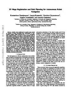
3 Path planning 3.1 A* algorithm The A* algorithm is a commonly used heuristic path planning algorithm that can be applied to find the shortest path from the start to the end of a grid map. The algorithm relies on the evaluation function 𝑓𝑓 𝑛𝑛 to measure whether the path is optimal. 𝑓𝑓 𝑛𝑛 = 𝑔𝑔 𝑛𝑛 + 𝑕𝑕(𝑛𝑛) (2) The evaluation function 𝑓𝑓 𝑛𝑛 is an evaluation function of node 𝑛𝑛, 𝑔𝑔 𝑛𝑛 represents the movement cost evaluation of node 𝑛𝑛 from the starting point, which is the movement distance of all the passed parent nodes by adding n to the starting point; 𝑕𝑕(𝑛𝑛)is cost to the end point, which is a heuristic value where the Manhattan distance is used to guide the algorithm to find the end point. As shown in Fig.3, the redletter S indicates the start node, the green letter E indicates the end node and the blue node indicates the found path. Algorithm pseudo-code shown in Fig.4.

4 Simulation and experimental 4.1 Mapping using LSD SLAM

The physical prototype used in this paper is omnidirectional wheel mobile platform. The physical prototype has three 60mm omnidirectional wheels driven by MD36 type 24V DC motor, self-developed CAN bus DC servo motor driver and open UART and CAN motion control interface to the upper computer equipment. Using HTPC industrial computerforimage progressing and obstacle avoidance calculation. Using MT9V034 type camera, global shutter, angle of view 140° , focal length 1.9mm, resolution 640 × 480 , frame rate 60Fps, complete visual collection; Using RPLIDAR A1 type Lidar, 360° scan, 6mmeasurement radius, the data acquisition frequency of 5.5HZ ,avoid obstacles. The overall electrical connection is shown in Fig.5(a), and the robot entity is shown in Figure Fig.5(b). Controlling the physical prototype to complete the loop-back motion in the indoor environment, as shown in Fig.6(a), the visual odometer calculates the pose change of 𝔰𝔰𝔢𝔢(3), and optimizes the map and Open FAB-Map to complete the loopback detection using 𝑔𝑔2 𝑜𝑜 . Finally, 639007 3D point cloud data are obtained, and an ASCII version of the polygon file format document (PLY) is saved. The obtained 3D point cloud map and the pose diagram of the physical prototype are shown in Fig.6(b).

Figure 3. A* algorithm find path.

In p u t : L ocation of S tart and E n d node O u tp u t : Father node of E nd 1. op en = list containing S tart node; 2. closed = em pty set; 3. m ovecost(x;y) = distance from node x to node y. 4. w h ile E n d node not in op en : d o 5. i = node w ith low est f(i) in op en ; 6. rem ove i from op en ; 7. add i to closed ; 8. count = 0; 9. for j = neighbor node of i an d not in closed an d reachable d o : 10. count+ + ; 11. cost = g(i)+ m ovecost(i;j); 12. if j in op en an d cost < g(j) th en : 13. rem ove j from op en ; 14. if j not in op en an d not in closed th en : 15. add j into op en ; 16. f(j) = g(j)+ h(j); 17. set father node of j is i; 18. if count = = 0 th en : 19. can't ¯nd path; 20. b reak ou t;

Figure 4. A* algorithm pseudo-code.

Figure 5 (a). Electrical Connection(b). Robot

3.2 A* algorithm performanceimprovement

4.2 Occupied grid mappreparation

3

MATEC Web of Conferences 160, 06004 (2018) https://doi.org/10.1051/matecconf/201816006004 MATEC Web of Conferences EECR 2018

After obtaining the PLY file, 364413 points cloud data are obtained according to STEP1 of Section 2.2, and then all the points are projected onto the ground to obtain a scattergram. Fig.7(a) is a path planning software interface running by the industrial computer.The software is based on OpenGL set up to achieve real-time display of 2-D terrain data, the number of horizontal grid is 168, the number of vertical grid is 120, the red point is the point of cloud projection, accounting for one pixel. Progressing the map according to STEP 2 and get the grid map as shown in Fig.7(b). The red area is not accessible and the green area is the accessible area. There are 8007 unacceptable grids and 121153 grids available.

Eff icie n cy co mp ariso n list

Dijkstra

168*120

336*240

0.09238

0.01385

0.03027

0.005451

0.05033

0.01265

0.00312

0.19324

0.3389

binary heap

672*480

Figure 9. Vertical axis is average of fifty different pairs of start node and end node summary time cost. Horizontal axis is three different maps. Orange is time cost of A* using binary heap data structure, yellow is time cost of A* using list data structure, green is time cost of Dijkstra algorithm.

Figure 6 (a). Indoor room(b). Point clouds map

5 Conclusions Inthis paper, the grid map preparation method and path planning strategy based on monocular vision simultaneous positioning and map construction are studied. The environment is reconstructed using the largescale direct method (LSD) model, which enables the environment to be accurately reconstructedin various scenarios of robots. Based on the environment threedimensional data, occupancy grid map (OGM) was prepared for the description of the terrain. According to the terrain information, A * algorithm was used for path planning, and the performance of the algorithm was improved. Simulation shows that the proposed method is more than 5 times faster than the traditional method. Next research will focus on controlling robot driving along the path and fixing robot pose according to VSLAM 𝔰𝔰𝔢𝔢(3) pose.

Figure 7 (a). Scatter plot(b). OGM.(c). Expansion OGM Then the expansion of the grid points is performed, using a Bresenham drawing circle algorithm from computer graphics--using a series of discrete points to approximate the circle and obtaining a grid expansion with a radius of 2 as shown in Fig.7(c). Radius can be dynamically adjusted

4.3 Path Planning Algorithm Simulation To evaluate the performance and performance of the A* algorithm, the algorithm was tested in the simulation software described above. The author first tests the performance of two data structure A* algorithms at different start node andend node on different size maps of 168 × 120,336 × 240,672 × 480,as shown in Fig.8(a) and (b). The yellow grid indicates the path to the plan. The letter S indicates the start node and the letter E indicates the end node. Fig.9 shows the comparison of the three methods at different fifty pairs of start node andend node. The vertical axis shows the fifty pairsaverage time.Unit issecond. It can be seen that the time cost of A* binary heap is about 1/5 of the A* list, while the Dijkstra algorithm has the longest time, ten times as much as the A* list.

References 1. 2. 3. 4.

5. 6. Figure 8 (a). West to east(b). North to south

4

E.W.Dijkstra, A Note on Two Problems inCinnexion with Graphs. Numerische Mathematik,1,269271,(1959). Amit Patel Introduction to A* ,1-28,(1997-10-16) Ferguson D,StentzA,Using interpolation to improve path planning: the field D algorithm. Journal of Field Robotics, 2006, 23( 2) : 79-101. XIN Yu,LIANG Huawei,DU Mingbo,MEI Tao, WANG Zhiling,JIANG Ruhai,An Improved A* Algorithm for Searching Infinite Neighbourhoods. Robot,(20-14),36(05):627-633. LI Chong,ZHANG An,BI Wenhao.Single-Boundary Rectangle Expansion A* Algorithm.Robot,2017,39 (01):46-56 XiangGao,TaoZhang,YiLiu,QinruiYan.Fourteen Lectures on Visual SLAM: From Theory to Practice

MATEC Web of Conferences 160, 06004 (2018) https://doi.org/10.1051/matecconf/201816006004 EECR 2018 EECR 2018

12. R. Wang, M. Schwörer, D. Cremers Stereo DSO: Large-Scale Direct Sparse Visual Odometry with Stereo Cameras , In International Conference on Computer Vision (ICCV), (2017) 13. V. Usenko, J. Engel, J. Stueckler, D. Cremers, Reconstructing Street-Scenes in Real-Time From a Driving Car , In Proc. of the Int. Conference on 3D Vision (3DV), (2015) 14. J. Engel, J. Stueckler, D. Cremers,Large-Scale Direct SLAM with Stereo Cameras , In-International Conference on Intelligent Robots and Systems (IROS), (2015) 15. Arren Glover,William Maddern,OpenFABMAP: An Open Source Toolbox for Appearance-based Loop Closure Detection,ICRA,14-18 May (2012)

[M]. Beijing: Publishing House of Electronics Industry, 2017: 130-137 7. Georg Klein, David Murray. Parallel Tracking and Mapping for Small AR Workspaces. In Proc. International Symposium on Mixed and Augmented Reality (ISMAR 2007, Nara) 8. Raúl Mur-Artal and Juan D. Tardós. ORB-SLAM2: an Open-Source SLAM System for Monocular, Stereo and RGB-D Cameras. IEEE Transactions on Robotics, vol. 33, no. 5, pp. 1255-1262, (2017) 9. J. Engel, J. Sturm, D. Cremers, Semi-Dense Visual Odometry for a Monocular Camera, J. Engel, J. Sturm, D. Cremers, ICCV (2013) 10. J. Engel, T. Schöps, D. Cremers, LSD-SLAM: Large-Scale Direct Monocular SLAM, ECCV(2014) 11. J. Engel, V. Koltun, D. Cremers.Direct Sparse Odometry , In arXiv:1607.02565, (2016)

5