Several non-exhaustive computational search tech- niques have .... to an ordered ranking factor of the rank-based se- lection within ..... Proceedings of the Florida Artificial Intelligence ... and Engineering Applications of Artificial Intel- ligence ...
Searching for Snake-in-the-Box Codes with Evolved Pruning Models Daniel R. Tuohy Stottler Henke Associates, Inc. San Mateo, CA
Walter D. Potter and Darren A. Casella Artficial Intelligence Center University of Georgia Athens, GA
achordal open paths (snakes) in n-dimensional hypercube graphs (the box). Our technique first obtains a set of exemplary snakes using an evolutionary algorithm. These snakes are then analyzed to define a pruning model that constrains the search space. A depth-first search of the constrained solution space has established new lower bounds for the length of the longest snakes in the 9 and 10 dimensional hypercube graphs.
0011 0001 1101 1001
1. An evolutionary algorithm is used to generate a set of very long snakes. 2. We compute several attributes of each snake at each node in the snake. 3. The upper and lower bounds of these attributes define a pruning model.
1110
1010
1000
0110
0100
0000
0010
Figure 1: A maximal length snake in Q4
Introduction
The snake-in-the-box problem is that of discovering the longest path in a hypercube graph such that the path is not adjacent to itself at any node. The longest such path for the dimension-4 hypercube is illustrated in Figure 1. For dimensions one through seven, longest maximal snakes have been found by exhaustive search techniques [7][15]. In higher dimensions, those greater than seven, the solution space is intractable. Several non-exhaustive computational search techniques have been employed to discover lengthy snakes in these dimensions, including genetic algorithms [16], distributed computing [11], neural networks [4], and other evolutionary algorithms [6]. We have developed a hybrid method described by this sequence of steps:
1111
1011
1100
Keywords: Search, Genetic Algorithms, Mathematics
1
0111
0101
Abstract We present a method for searching for
4. We perform a depth first search of all snakes, pruning and backtracking whenever any attribute of the current snake escapes the model. The reader should note that we are not concerned with time efficiency. We are interested only in obtaining snakes which are longer than the current theoretical lower bound, and therefore have not yet been discovered either through computational search or mathematical construction. We have achieved this objective for the 9 and 10 dimensional hypercube graphs.
2
Applications
The snake-in-the-box problem was first described in a paper by Kautz in the late 1950s, and was noted for its relevance to coding theory [12]. Snake-inthe-box codes are useful because they are “spread 2” gray codes. This means that any two codewords are at least two entries apart in the list of codewords or that they differ in at least two positions. Consequently, errors at only one position (the most common case) are easily detectable because they will reference code words at positions in the list which
are more obviously inappropriate [10]. Snakes have been put to use in disjunctive normal form simplification, electronic combination locking mechanisms, disk sector encoding, and analog-to-digital conversion [14][13][5][15][8]. The specific use of snake-in-the-box codes in these domains is often error-detection and correction, and the longest snakes are the most useful for this purpose. Consequently, methods for discovering the longest snakes in dimensions eight and above have been the subject of much research in both mathematics and computer science (See references).
3
Dimension
n-snake
n-coil
Q1 Q2 Q3 Q4 Q5 Q6 Q7 Q8 Q9 Q10 Q11 Q12
1 2 4 7 13 26 50 97 186 358 680 1260
2 4 6 8 14 26 48 96 180 344 630 1238
Background and Terminology
Table 1: Longest snakes and coils in Qn . For n≥8, solutions are only the current best-known.
Following standard convention, we use Qn to denote the n-dimensional hypercube, which is defined inductively as the Cartesian product of Q1 and Qn−1 . It is useful to think of Q1 as a line (two constituent nodes), Q2 as a square (four), Q3 as a cube (eight), and Q4 as the sixteen-node graph in Figure 1. For n>4, meaningful visualisation is tricky. There are 2n nodes in Qn that can be represented as vectors of binary digits. The nodes are labeled in such a way that the binary vectors of adjacent nodes always differ by exactly one bit, as in Figure 1. An induced path in Qn , as defined in [9], is a sequence of nodes P such that for any u,v∈P, if u and v are adjacent in Qn then they are also adjacent in P. A path is expressed in node sequence representation if it is a vector of base-10 integers corresponding to the binary labels on each node in the path. The node sequence of the snake in Figure 1 is {0 1 3 7 6 14 12 13}. A path is expressed in transition sequence representation if it is a vector of integers in the range 0..n-1 [1]. These integers correspond to the index of the bit in the bit string that was flipped to grow the snake from one node to the next. The index of the least significant bit is 0 and that of the most significant bit is n-1. The transition sequence of the snake in Figure 1 is {0 1 2 0 3 1 0}. The term “Snake in the Box” (derived from the visualization of a chain as a unit-radius tube) originally designated induced cycles, or closed paths (also called closed chains), in a graph [12]. We adopt the terminology introduced in [9], who assign the term “coil” to simple cycles and the term
“n-coil” to coils of maximal length in Qn . The terms “snake” and “n-snake” are used in exactly the same way to designate induced open paths. The lengths of n-snakes and n-coils up to n = 6 were computed via exhaustive search by Davies [7]. Those for n = 7 were determined by the Genetic Algorithm of Potter [16] and later the exhaustive technique of Kochut [15], which we will be building upon. Table 1 shows the lengths of the n-snakes and n-coils for n≤7, as well as current best-known lengths of longest snakes and coils in dimensions 8 through 12 [2][6][7][9][15][16].
4
PBSHC: An Evolutionary Algorithm for Obtaining Model Snakes
A Population-Based Stochastic Hill-Climber (PBSHC) was used to generate our model snakes. This algorithm is described in more detail in [6]. The PBSHC evolves a population of snakes from a zero or small initial length to some maximum length. Each individual in the population consists of a sequence of integers that represents the node sequence of a snake, or valid path through the hypercube, in the dimension being searched. These individuals are initialized as either a snake of length zero, that is consisting of only the zero node, or seeded with a pre-existing snake of choice. Following initialization, the evolutionary cycle begins its first generation. Each generation begins with a fitness evaluation. The fitness function used is based on both the length and the ‘tightness’ of the snake. The tightness of a snake, as defined for the PBSHC,
is a measure of how many nodes are left available in the hypercube after subtracting all those nodes that are disqualified either by already being in the snake or by being adjacent to another node in the snake. The choice of tightness as a component of the fitness function was inspired by the idea that tighter snakes, since they make more efficient use of nodes, might have more room to grow. Initial attempts of integrating both length and tightness into a fitness function met with limited success. Many combinations of linear and nonlinear factors of length and tightness for the fitness function were tried. While they each performed well in some periods of evolution, they would inevitably perform worse in others. Once the average fitness of the population slowed, the diversity of the population would fall and the fitness function would converge to a local optimum. Our first attempt at solving this problem was to develop an adaptive fitness function that would balance between the importance of tightness and length, using the diversity of the population as the balancing factor. This technique also met with limited success, reacting to changes in diversity too quickly in some cases and not quickly enough in others. Our second attempt was a more simplistic compromise between the two objectives. Length was set as the overriding objective within each generation, and tightness delegated to an ordered ranking factor of the rank-based selection within each generation. Since all snakes that were able to grow in the previous generation have the same length in the current generation, tightness becomes the only distinguishing factor of the fitness function. After the individual fitness of each of the snakes in the population is determined, the population is subjected to rank-based selection based upon each snake’s fitness. In order to keep the population constant throughout the entire run, the remaining places available in the population of the next generation are filled starting again with the most fit individuals. For example, if the selection percentage is 90%, the individuals are ranked by fitness and the first 90% are selected. This still leaves 10% of the next generation empty, so the first 10% from the current generation are used to finish the selection operation. After selection, the growth operator grows each snake in the population by one step each generation, connecting each snake’s end node to one of its adjacent nodes that has not been disqualified by already being in the snake, or by being adjacent to some node that is in the snake. While bi-directional growth was used during preliminary trials in dimen-
sion eight, unidirectional growth was chosen for this implementation to best allocate computational resources. This operator can be seen to perform a stochastic hill-climbing process on each snake in the population as the choice of which adjacent node to connect to is based on random selection from the available nodes. A choice was made early to grow all snakes in the population instead of only the snake of best fitness (note: enhancing the best individual in a population is a common approach in hybrid genetic algorithms). This choice was also based on results of a comparison of these two approaches in an earlier GA implementation. Growing all the individuals within the population also works well in conjunction with the fitness function which requires that all snakes in the population of a given generation be of the same length in order to function properly. The fitness function consists of the sum of the snake’s length and normalized tightness. This results in the fitness function simplifying to a function of tightness alone as the length component of the fitness value will dominate for snakes of different lengths, yet cancel for snakes of the same length. This also results in the automatic elimination of snakes that can no longer grow, allowing their place in the population to be reallocated to other snakes that are still capable of growth. The choice of parameter settings was found to be of key importance to the performance of the PBSHC and these settings were tuned extensively in dimension eight before modified to run in dimensions nine and above. Our previous experience with genetic algorithm snake hunters supported the application of lower-dimension parameter settings as a baseline for higher-dimension runs. The fitness function is set to the sum of length and normalized tightness. Normalized tightness was defined as the number of nodes remaining available divided by the total number of nodes in the n-dimensional hypercube. Rank-based selection was chosen in order to maximize diversity within the population. While both unidirectional and bi-directional growth were used in the dimension-eight trials, the relatively memory-conservative, unidirectional implementation was chosen for the higher-dimensional runs in order to maximize potential population sizes for dimensions nine and above. Because this particular implementation’s chromosome size is constant, the use of unidirectional growth instead of bi-directional growth allowed the required memory for each population size to be reduced by half. Population sizes from one hundred through ten thousand were run in trials using mutation. The best results were achieved using popula-
tions of ten thousand, a selection percentage of ninety percent, and by seeding each population with highly-fit snakes from a lower-dimension. For the purposes of the method described in this paper, we have used PBSHC to generate a set of very long snakes in dimensions 9 and 10.
dimension 9, by only searching for snakes in canonical form we eliminate 99.9997% (n!-1 /n! ) of the solution space from consideration.
5
The solution space afforded by Kochut’s approach is still far too massive to be searched exhaustively in dimensions greater than 7. We therefore introduce further constraints that no longer guarantee the maximal length snake will be found. Consequently, we can only find new lower bounds for maximal snake lengths, rather than absolute bounds. The following three constraints ensure that every snake considered in the depth first search adheres to a set of parameter boundaries defined by the model snakes found via PBSHC. In essence, we are making a much more strict definition of a “dead end” in the search. Backtracking now occurs not only when there are no available adjacent nodes, but also when all available nodes cause the snake to escape the parameter boundaries. Tightness. We have defined tightness as the degree to which different nodes in the snake render identical nodes inaccessible and is proportional to the number of pairs of included nodes with a hamming distance of 2. For example, nodes 000000000 and 000000011 both render node 000000001 inaccessible because they differ at exactly 2 bits. The “tighter” a snake is wound, the more nodes remain available at each step in the snake. We express tightness as “the number of unavailable nodes per node in the snake”. If there are 18 unavailable nodes at node 4 in the snake, the tightness of the snake is 4.5. It tends to be desirable to keep this number low. However, we have found that our model snakes do not always choose the tightest possible path at every step. We therefore prune branches both when snakes are too loose and when they are too tight. Figure 2 is an example of tightness boundaries that have been defined by model snakes in Dimension 9. Tightness Rate-of-change. Consider a snake that is on the tighter edge of the tightness boundary defined by our model snakes at the kth step in the snake. For the next several steps, the search has license to take inadvisable turns that needlessly eat up available nodes in the hypercube since it will still stay inside the tightness boundary. To eliminate this possibility, we only allow a snake’s tightness to increase or decrease at a certain rate. We do this by extracting the “percent change in tightness over the last 5 steps” at each step in our model
Constraining the Solution Space for a Depth-First Search
To explore the solution space, we attempt to grow a snake until it reaches a dead end. The search then backtracks until further progress can be made in a different direction. This process is repeated until every snake has been explored. Unfortunately, there are far too many possible snakes to try every one, and we are forced to constrain the solution space artificially. We will describe five methods by which we constrain the solution space so that it may be fully explored by a depth first search. The first two, described in the following section, were first implemented by Kochut for exploring Q7 .
5.1
Kochut’s Constraints
The constraints implemented by Kochut are independent of model snakes and were first used in an exhaustive snake searching algorithm devised for the dimension 7 hypercube. Neither of these restrictions can possibly prevent the discovery of a maximal length snake, yet they drastically increase search efficiency. Always begin at node 0. To understand why this does not prevent us from finding possible maximal length snakes, it is helpful to consider a snake in transition sequence (see Sect. 3). From a snake starting at node 0 in Qn , one can obtain 2n identical snakes in node sequence simply by applying the corresponding transition sequence beginning at every node in Qn . In dimension 9, by only searching for snakes originating at node 0 we eliminate 99.8% (2n -1/2n ) percent of the solution space from consideration. Only consider snakes in canonical form. Snakes in canonical form are those which only use higherorder dimensions after every lower-order dimension has been used at least once. Hypercubes have n! symmetries, and canonical form is but one of these. Again, consider a snake in transition sequence. By swapping, say, all of the 8’s and 1’s, we obtain an identical snake with a different node sequence. It simply uses the dimensions in a different order. In
5.2
Constraints Based Snakes
on Model
Tightness Pruning Boundaries 10
Unavailable nodes/node in the snake
9 8 7 6
6
5
Results
4 3 2 1
13 25 37 49
61 73 85 97 109 121 133 145 157 169 181 Node in the snake
Figure 2: The tightness boundaries defined by the model snakes found via PBSHC. Snakes are pruned as soon as they escape these boundaries. Tightness Rate-of-change Pruning Boundaries
%change in tightness over the last 5 nodes
sion 4 is always the most used dimension. Each dimension has a range of about 10 uses from which it never deviates in the model snakes. Currently, we only prune snakes which overuse any of the dimensions and do not prune for underuse.
19
14
We have two methods of control over how strictly we constrain the solution space. The first is choosing a seed snake. Past research has found it useful to choose a portion of a best known snake from a lower dimension to seed a search algorithm [6]. A seed, in effect, sets in stone the initial section of the path. A seed of 37 nodes, for example, decides the path through the highest 37 levels of the search tree. This reduces the solution space considerably. The second is the number of snakes used to define the pruning model. Fewer snakes intuitively results in narrower pruning boundaries because there is less variability among fewer snakes.
9
6.1
4
-1
1
12 23 34
45 56 67
78 89 100 111 122 133 144 155 166 177188 Node in snake
Figure 3: The tightness rate-of-change boundaries defined by the model snakes found via PBSHC. Snakes are pruned as soon as they escape these boundaries. snakes. This corresponds to the rate of change in tightness at each step, and we do not allow snakes to tighten or loosen faster than any of the model snakes. Figure 3 shows the tightness rate-of-change boundaries that have been define by model snakes. Maximal Dimension Cumulative Usage. This term refers to the number of times each dimension has been “used” in the snake, and was first described by Bishop [3]. A dimension is “used” if it has been flipped from a 1 to a 0 or vice-versa in the course of creating the path. Usage is equivalent to the number of occurrences in the transition sequence. We have observed a great deal of homogeneity in the Dimension Cumulative Usage of model snakes. This is in part due to the fact that all model snakes are in canonical form, which ensures that the dimensions are ordered the same way. In the Q9 model snakes, the highest dimension is always used only once. Additionally, dimension 6 is always used more than dimension 5 and dimen-
Dimension 9
A base of 344 snakes was built using the Evolutionary Algorithm described in section 4 to define the pruning model. Our depth first search was given a seed snake of length 37 from a maximal length snake in dimension 8, which can be found in [17]. The seed was neccessary to provide a search space that could be searched exhaustively. An exhaustive search with pruning from the 38th node yielded five new snakes of length 188. One of these snakes, in transition sequence notation: 01234532103253123452310326 054301350231035430137413015 201305413062103453013205310 345263026123678632052103453 013205310345263025345031025 103124765231036203102562134 503102356250213025012613463 This constitutes an improvement over the previous lower bound of 186.
6.2
Dimension 10
Because the solution space for Q10 is exponentially bigger than that of Q9 , we were forced to constrain the solution space more harshly. The pruning model was defined using only 30 snakes found by the Evolutionary Algorithm, and we used the first 185 nodes of the best known Q9 snake (listed above) to seed the depth first search. It should
be noted that our search of the constrained solution space was not exhaustive. After two weeks of runtime, two snakes of length 363 were found (the search proceeded for several more weeks without termination or improvement). One of these snakes, in transition sequence notation: 01234532103253123452310326 054301350231035430137413015 201305413062103453013205310 345263026123678632052103453 013205310345263025345031025 103124765231036203102510364 316210520312052653201305431 953402310250345263025345031 025103143610318453201325316 532053152354315201560352301 325673621034530135613015201 305435682013250145031023562 502130250126134630152013028 0625430135423 This constitutes an improvement over the previous lower bound of 358. For both dimensions 9 and 10, the new lower bounds represent greater than 1% improvement over previous lower bounds.
[4] Bishop, J. 2006. Investigating the snake-inthe-box problem with neuroevolution. Dept. of Computer Science, The University of Texas at Austin. Forthcoming.
7
[10] Hiltgen, A., and Paterson, K. 2000. Singletrack circuit codes. IEEE Transactions on Information Theory 47(6):2587–2595.
Conclusion
We intend to expand the search technique to the hypercubes of higher dimensions. In addition, we shall adapt the search to be applied to the problem of finding lengthy coils. We have no reason to believe that the search will not work equally well on these problems, and hope that further lower bounds will be established. It is likely that our method would benefit from further pruning heuristics. The three described in this paper are simply those which seemed most relevant, and more informative measures may well exist.
References [1] Abbott, H., and Katchalski, M. 1988. On the snake in the box problem. Journal of Combinatorial Theory 45:13–24.
[5] Blaum, M., and Etzion, T. 2002. Use of snake-in-the-box codes for reliable identification of tracks in servo fields of a disk drive. U.S. patent 6496312. [6] Casella, D., and Potter, W. 2005. New lower bounds for the snake-in-the-box problem: Using evolutionary techniques to hunt for snakes. In Proceedings of the Florida Artificial Intelligence Research Society Conference. [7] Davies, D. 1965. Longest ’separated’ paths and loops in an n cube. IEEE Trans. Electron. Comput. 14:261. [8] Etzion, T., and Paterson, K. 1996. Near optimal single-track gray codes. IEEE Trans. Inform. theory. 42:779–789. [9] Harary, F.; Hayes, J.; and Wu, H. 1988. A survey of the thoery of hypercube graphs. Computational Mathematics Applications 40:277–289.
[11] Juric, M.; Potter, W.; and Plaskin, M. 1994. Using pvm for hunting snake-in-the-box codes. In Proceedings of the Transputer Research and Applications Conference, 97–102. [12] Kautz, W. 1958. Unit-distance error-checking codes. IRE Trans. Elecronic Computers 7:179– 180. [13] Klee, V. 1970a. The use of circuit codes in analog-to-digital conversion. In Graph Theory and its Applications. B. Harris, ed. New York, NY: Academic Press. [14] Klee, V. 1970b. What is the maximum length of a d-dimensional snake? American Mathematics Monthly 77:63–65.
[2] Abbott, H., and Katchalski, M. 1991. On the construction of snake-in-the-box codes. Utilitas Mathematica 40:97–116.
[15] Kochut, K. 1996. Snake-in-the-box codes for dimension 7. Journal of Combinatorial Mathematics and Combinatorial Computations 20:175– 185.
[3] Bishop, J. 2004. Snake hunting by genetic construction. Technical report, Artificial Intelligence Center, The University of Georgia.
[16] Potter, W.; Robinson, R.; Miller, J.; and Kochut, K. 1994. Using the genetic algorithm to find snake-in-the-box codes. In Proceedings of
the 7th International Conference On Industrial and Engineering Applications of Artificial Intelligence, 421–426. [17] Rajan, D., and Shende, A. 1999. Maximum and reversible snakes in hypercubes. In Proceedings of the Annual Australasian Conference on Combinatorial Mathematics and Combinatorial Computation.