Second-Order Polynomial Models for Background ... - Semantic Scholar

Second-Order Polynomial Models for Background Subtraction Alessandro Lanza, Federico Tombari, Luigi Di Stefano DEIS, University of Bologna Bologna, Italy {alessandro.lanza, federico.tombari, luigi.distefano }@unibo.it

Abstract. This paper is aimed at investigating background subtraction based on second-order polynomial models. Recently, preliminary results suggested that quadratic models hold the potential to yield superior performance in handling common disturbance factors, such as noise, sudden illumination changes and variations of camera parameters, with respect to state-of-the-art background subtraction methods. Therefore, based on the formalization of background subtraction as Bayesian regression of a second-order polynomial model, we propose here a thorough theoretical analysis aimed at identifying a family of suitable models and deriving the closed-form solutions of the associated regression problems. In addition, we present a detailed quantitative experimental evaluation aimed at comparing the different background subtraction algorithms resulting from theoretical analysis, so as to highlight those more favorable in terms of accuracy, speed and speed-accuracy tradeoff.

1

Introduction

Background subtraction is a crucial task in many video analysis applications, such as e.g. intelligent video surveillance. One of the main challenges consists in handling disturbance factors such as noise, gradual or sudden illumination changes, dynamic adjustments of camera parameters (e.g. exposure and gain), vacillating background, which are typical nuisances within video-surveillance scenarios. Many different algorithms for dealing with these issues have been proposed in literature (see [1] for a recent survey). Popular algorithms based on statistical per-pixel background models, such as e.g. Mixture of Gaussians (MoG) [2] or kernel-based non-parametric models [3], are effective in case of gradual illumination changes and vacillating background (e.g. waving trees). Unfortunately, though, they cannot deal with those nuisances causing sudden intensity changes (e.g. a light switch), yielding in such cases lots of false positives. Instead, an effective approach to tackle the problem of sudden intensity changes due to disturbance factors is represented by a priori modeling over small image patches of the possible spurious changes that the scene can undergo. Following this idea, a pixel from the current frame is classified as changed if the intensity transformation between its local neighborhood and the corresponding neighborhood in the background can not be explained by the chosen a priori

2

A. Lanza, F. Tombari, L. Di Stefano

model. Thanks to this approach, gradual as well as sudden photometric distortions do not yield false positives provided that they are explained by the model. Thus, the main issue concerns the choice of the a priori model: in principle, the more restrictive such a model, the higher is the ability to detect changes (sensitivity) but the lower is robustness to sources of disturbance (specificity). Some proposals assume disturbance factors to yield linear intensity transformations [4, 5]. Nevertheless, as discussed in [6], many non-linearities may arise in the image formation process, so that a more liberal model than linear is often required to achieve adequate robustness in practical applications. Hence, several other algorithms adopt order-preserving models, i.e. assume monotonic non-decreasing (i.e. non-linear) intensity transformations [6–9]. Very recently, preliminary results have been proposed in literature [10, 11] that suggest how second-order polynomial models hold the potential to yield superior performance with respect to the classical previously mentioned approaches, being more liberal than linear proposals but still more restrictive than the order preserving ones. Motivated by these encouraging preliminary results, in this work we investigate on the use of second-order polynomial models within a Bayesian regression framework to achieve robust background subtraction. In particular, we first introduce a family of suitable second-order polynomial models and then derive closed-form solutions for the associated Bayesian regression problems. We also provide a thorough experimental evaluation of the algorithms resulting from theoretical analysis, so as to identify those providing the highest accuracy, the highest efficiency as well as the best tradeoff between the two.

2

Models and solutions T

T

For a generic pixel, let us denote as x = (x1 , . . . , xn ) and y = (y1 , . . . , yn ) the intensities of a surrounding neighborhood of pixels observed in the two images under comparison, i.e. background and current frame, respectively. We aim at detecting scene changes occurring in the pixel by evaluating the local intensity information contained in x and y. In particular, classification of pixels as changed or unchanged is carried out by a priori assuming a model of the local photometric distortions that can be yielded by sources of disturbance and then testing, for each pixel, whether the model can explain the intensities x and y observed in the surrounding neighborhood. If this is the case, the pixel is likely sensing an effect of disturbs, so it is classified as unchanged; otherwise, it is marked as changed. 2.1

Modeling of local photometric distortions

In this paper we assume that main photometric distortions are due to noise, gradual or sudden illumination changes, variations of camera parameters such as exposure and gain. We do not consider here the vacillating background problem (e.g. waving trees), for which the methods based on multi-modal and temporally adaptive background modeling, such as [2] and [3], are more suitable.

Second-Order Polynomial Models for Background Subtraction

3

As for noise, first of all we assume that the background image is computed by means of a statistical estimation over an initialization sequence (e.g. temporal averaging of tens of frames) so that noise affecting the inferred background intensities can be neglected. Hence, x can be thought of as a deterministic vector of noiseless background intensities. As for the current frame, we assume that noise is additive, zero-mean, i.i.d. Gaussian with variance σ 2 . Hence, noise affecting the vector y of current frame intensities can be expressed as follows: p(y|˜ y) =

n Y i=1

p(yi |˜ yi ) =

n ´−n ³ ´ ¡ ¢ ³√ 1 X 2πσ exp − 2 (yi − y˜i )2 (1) N y˜, σ 2 = 2σ i=1 i=1 n Y

T

˜ = (˜ where y y1 , . . . , y˜n ) denotes the (unobservable) vector of current frame noiseless intensities and N (µ, σ 2 ) the normal pdf with mean µ and variance σ 2 . As far as remaining photometric distortions are concerned, we assume that noiseless intensities within a neighborhood of pixels can change due to variations of scene illumination and of camera parameters according to a second-order polynomial transformation φ(·), i.e.: y˜i = φ (xi ; θ) = (1, xi , x2i ) (θ0 , θ1 , θ2 )T = θ0 + θ1 xi + θ2 xi 2

∀ i = 1, . . . , n (2)

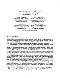
It is worth pointing out that the assumed model (2) does not imply that the whole frame undergoes the same polynomial transformation but, more generally, that such a constraint holds locally. In other words, each neighborhood of intensities is allowed to undergo a different polynomial transformation, so that local illumination changes can be dealt with. From (1) and (2) we can derive the expression of the likelihood p(x, y|θ), that is the probability of observing the neighborhood intensities x and y given a polynomial model θ: n ´−n ³ 1 X ´ 2 2πσ exp − 2 (yi − φ(xi ; θ)) 2σ i=1 (3) where the first equality follows from the deterministic nature of the vector x that allows to treat it as a vector of parameters. In practice, not all the polynomial transformations belonging to the linear space defined by the assumed model (2) are equally likely to occur. In Figure (1), on the left, we show examples of less (in red) and more (in azure) likely transformations. To summarize the differences we can say that the constant term of the polynomial has to be small and that the polynomial has to be monotonic non-decreasing. We formalize these constraints by imposing a prior probability on the parameters vector θ = (θ0 , θ1 , θ2 )T , as illustrated in Figure (1), on the right. In particular, we implement the constraint on the constant term by assuming a zero-mean Gaussian prior with variance σ02 for the parameter θ0 :

p(x, y|θ) = p(y|θ; x) = p(y|˜ y = φ(x; θ)) =

³√

p(θ0 ) = N (0, σ02 )

(4)

The monotonicity constraint is addressed by assuming for (θ1 , θ2 ) a uniform prior inside the subset Θ12 of R2 that renders φ0 (x; θ) = θ1 + 2θ2 · x ≥ 0 for all

4

A. Lanza, F. Tombari, L. Di Stefano ∂

   ≥ 





    N 

Θ









 






 

∂  
     ≤ 

Fig. 1. Some polynomial transformations (left, in red) are less likely to occur in practice than others (left, in azure). To account for that, we assume a zero-mean normal prior for θ0 , a prior that is uniform inside Θ12 , zero outside for (θ1 ,θ2 ) (right).

x ∈ [0 , G], with G denoting the highest measurable intensity (G = 255 for 8-bit images), zero probability outside Θ12 . Due to linearity of φ0 (x), the monotonicity constraint φ0 (x; θ) ≥ 0 over the entire x-domain [0 , G] is equivalent to impose monotonicity at the domain extremes, i.e. φ0 (0; θ) = θ1 ≥ 0 and φ0 (G; θ) = θ1 + 2G · θ2 ≥ 0. Hence, we can write the constraint as follows: © ª ½ k if (θ1 , θ2 ) ∈ Θ12 = (θ1 , θ2 ) ∈ R2 : θ1 ≥ 0 ∧ θ1 + 2Gθ2 ≥ 0 p(θ1 , θ2 ) = (5) 0 otherwise We thus obtain the prior probability of the entire parameters vector as follows: p(θ) = p(θ0 ) · p(θ1 , θ2 )

(6)

In this paper we want to evaluate six different background subtraction algorithms, relying on as many models for photometric distortions obtained by combining the assumed noise and quadratic polynomial models in (1) and (2), that imply (3), with the two constraints in (4) and (5). In particular, the six considered algorithms (Q stands for quadratic) are: Q∞ Qf Q0 Q ∞, M Q f, M Q 0, M 2.2

: : : : : :

(1) ∧ (2) ⇒ (3) plus prior (4) for θ0 with σ02 → ∞ (θ0 free); (1) ∧ (2) ⇒ (3) plus prior (4) for θ0 with σ02 finite positive; (1) ∧ (2) ⇒ (3) plus prior (4) for θ0 with σ02 → 0 (θ0 = 0); same as Q ∞ plus prior (5) for (θ1 , θ2 ) (monotonicity constraint); same as Q f plus prior (5) for (θ1 , θ2 ) (monotonicity constraint); same as Q 0 plus prior (5) for (θ1 , θ2 ) (monotonicity constraint);

Bayesian polynomial fitting for background subtraction

Independently from the algorithm, scene changes are detected by computing a measure of the distance between the sensed neighborhood intensities x, y and the space of models assumed for photometric distortions. In other words, if the intensities are not well-fitted by the models, the pixel is classified as changed. The minimum-distance intensity transformation within the model space is computed by a maximum a posteriori estimation of the parameters vector: θ MAP = argmax p(θ|x, y) = argmax [p(x, y|θ)p(θ)] θ ∈ R3 θ ∈ R3

(7)

Second-Order Polynomial Models for Background Subtraction

5

where the second equality follows from Bayes rule. To make the posterior in (7) explicit, an algorithm has to be chosen. We start from the more complex one, i.e. Q f, M . By substituting (3) and (4)-(5), respectively, for the likelihood p(x, y|θ) and the prior p(θ) and transforming posterior maximization into minus log-posterior minimization, after eliminating the constant terms we obtain: n h i X 2 θ MAP = argmin E(θ; x, y) = d(θ; x, y) + r(θ) = (yi − φ(xi ; θ)) + λθ02 (8) θ∈Θ i=1

The objective function to be minimized E(θ; x, y) is the weighted sum of a data-dependent term d(θ; x, y) and a regularization term r(θ) which derive, respectively, from the likelihood of the observed data p(x, y|θ) and the prior of the first parameter p(θ0 ). The weight of the sum, i.e. the regularization coefficient, depends on both the likelihood and the prior and is given by λ = σ 2 /σ02 . The prior of the other two parameters p(θ1 , θ2 ) expressing the monotonicity constraint has translated into a restriction of the optimization domain from R3 to Θ = R × Θ12 . It is worth pointing out that the data dependent term represents the least-squares regression error, i.e. the sum over all the pixels in the neighborhood of the square differences between the frame intensities and the background intensities transformed by the model. By making φ(xi ; θ) explicit and after simple algebraic manipulations, it is easy to observe that the objective function is quadratic, so that it can be compactly written as: E(θ; x, y) = (1/2) θ T H θ − bT θ + c with the matrix H, the  N  H = 2 Sx Sx2

vector b and the scalar c given by:    Sx Sx2 Sy Sx2 Sx3  b = 2 Sxy  3 4 Sx Sx Sx2 y

(9)

c = Sy 2

(10)

N = n+λ

(11)

and, for simplicity of notation: Sx = Sy =

n X i=1 n X i=1

2

xi Sx = yi Sxy =

n X i=1 n X i=1

x2i

3

Sx =

xi yi Sx2 y =

n X i=1 n X i=1

x3i

4

Sx =

x2i yi Sy 2 =

n X i=1 n X

x4i yi2

i=1

As for the optimization domain Θ = R × Θ12 , with Θ12 defined in (5) and illustrated in Figure 1, it also can be compactly written in matrix form as follows: ¶ µ © ª 0 1 0 3 (12) Θ = θ ∈R : Zθ ≥0 with Z= 0 1 2G The estimation problem (8) can thus be written as a quadratic program: £ ¤ θ MAP = argmin (1/2) θ T H θ − bT θ + c Zθ ≥0

(13)

6

A. Lanza, F. Tombari, L. Di Stefano

If in the considered neighborhood there exist three pixels characterized by different background intensities, i.e. ∃ i, j, k : xi 6= xj 6= xk , it can be demonstrated that the matrix H is positive-definite. As a consequence, since H is the Hessian of the quadratic objective function, in this case the function is strictly convex. Hence, it admits a unique point of unconstrained global minimum θ (u) that can be easily calculated by searching for the unique zero-gradient point, i.e. by solving the linear system of normal equations: θ (u) = θ ∈ R3 :

∇E(θ) = 0

≡

(H/2) θ = (b/2)

(14)

for which a closed-form solution is obtained by computing the inverse of H/2:    A D E Sy 1 D B F  Sxy  θ (u) = (H/2)−1 (b/2) = (15) |H/2| E F C Sx2 y where: ¡ ¢2 A = Sx2 Sx4 − Sx3

¡ ¢2 B = N Sx4 − Sx2 ¡ ¢2 E = Sx Sx3 − Sx2

D = Sx2 Sx3 − Sx Sx4 and

C = N Sx2 − (Sx)

2

F = Sx Sx2 − N Sx3

|H/2| = N A + Sx D + Sx2 E

(16)

(17) (u)

If the computed point of unconstrained global minimum θ belongs to the quadratic program feasible set Θ, i.e. satisfies the monotonicity constraint Z θ ≥ 0, then the minimum distance between the observed neighborhood intensities and the model of photometric distortions is simply determined by substituting θ (u) for θ in the objective function. A compact close-form expression for such a minimum distance can be obtained as follows: T

T

T

T

E (u) = E(θ (u) ) = θ (u) (H/2) θ (u) − θ (u) b + c = θ (u) (b/2) − θ (u) b + c ¢ T −1 ¡ = c − θ (u) (b/2) = Sy 2 − |H/2| Sy θ0(u) + Sxy θ1(u) + Sx2 y θ2(u) (18) The two algorithms Q f and Q ∞ rely on the computation of the point of unconstrained global minimum θ (u) by (15) and, subsequently, of the unconstrained minimum distance E (u) = E(θ (u) ) by (18). The only difference between the two algorithms is the value of the pre-computed constant N = n + λ that in Q ∞ tends to n due to σ02 → ∞ causing λ → 0. Actually, Q f corresponds to the method proposed in [10]. If the point θ (u) falls outside the feasible set Θ, the solution θ (c) of the constrained quadratic programming problem (13) must lie on the boundary of the feasible set, due to convexity of the objective function. However, since the monotonicity constraint Z θ ≥ 0 does not concern θ0 , again the partial derivative of the objective function with respect to θ0 must vanish in correspondence of the solution. Hence, first of all we impose this condition, thus obtaining: ¡ ¢ θ0 (c) = (1/N ) Sy − θ1 Sx − θ2 Sx2 (19)

Second-Order Polynomial Models for Background Subtraction

7

We thus substitute θ0 (c) for θ0 in the objective function, so that the original 3-d problem turns into a 2-d problem in the two unknowns θ1 , θ2 with the feasible set Θ12 defined in (5) and illustrated in Figure 1, on the right. As previously mentioned, the solution of the problem must lie on the boundary of the feasible set ∂Θ12 , that is on one of the two half-lines: ∂Θ1 : θ1 = 0 ∧ θ2 ≥ 0

∂Θ2 : θ1 = − 2 G θ2 ∧ θ2 ≤ 0

(20)

The minimum of the 2-d objective function on each of the two half-lines can be determined by replacing the respective line equation into the objective function and then searching for the unique minimum of the obtained 1-d convex quadratic function in the unknown θ2 restricted, respectively, to the positive (∂Θ1 ) and the negative (∂Θ2 ) axis. After some algebraic manipulations, we obtain that the (c) (c) two minimums E1 and E2 are given by:  2  2 2  T 2  V (Sy) (Sy) if T > 0 if V < 0 (c) (c) E1 = Sy 2 − − NB E2 = Sy 2 − − NU   N N 0 if T ≤ 0 0 if V ≥ 0 (21) where: T = N Sx2 y − Sx2 Sy V = T + 2GW (22) W = SxSy − N Sxy U = B + 4G2 C + 4G F (c)

The constrained global minimum E (c) is thus the minimum between E1 and (c) E2 . Hence, similarly to Q f and Q ∞ , the two algorithms Q f, M and Q ∞, M rely on the preliminary computation of the point of unconstrained global minimum θ (u) by (15). However, if the point does not satisfy the monotonicity constraint in (12), the minimum distance is computed by (21) instead of by (18). The two algorithms Q f, M and Q ∞, M differ in the exact same way as Q f and Q ∞ , i.e. only for the value of the pre-computed parameter N . The two remaining algorithms, namely Q 0 and Q 0, M , rely on setting σ02 → 0. This implies that λ → ∞ and, therefore, N = (n + λ) → ∞. As a consequence, closed-form solutions for these algorithms can not be straightforwardly derived from the previously computed formulas by simply substituting the value of N . However, σ02 → 0 means that the parameter θ0 is constrained to be zero, that is the quadratic polynomial model is constrained to pass through the origin. Hence, closed-form solutions for these algorithms can be obtained by means of the same procedure outlined above, the only difference being that in the model (2) θ0 has to be eliminated. Details of the procedure and solutions can be found in [11]. By means of the proposed solutions, we have no need to resort to any iterative approach. In addition, it is worth pointing out that all terms involved in the calculations can be computed either off-line (i.e. those involving only background intensities) or by means of very fast incremental techniques such as Summed Area Table [12] (those involving also frame intensities). Overall, this allows the proposed solutions to exhibit a computational complexity of O(1) with respect to the neighborhood size n.

8

A. Lanza, F. Tombari, L. Di Stefano

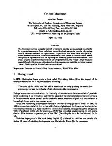
Fig. 2. Top: AUC values yielded by the evaluated algorithms with different neighborhood sizes on each of the 5 test sequences. Bottom: average AUC (left) and FPS (right) values over the 5 sequences.

3

Experimental results

This Section proposes an experimental analysis aimed at comparing the 6 different approaches to background subtraction based on a quadratic polynomial model derived in previous Section. To distinguish between the methods we will use the notation described in the previous Section. Thus, e.g., the approach presented in [10] is referred to here as Qf , and that proposed in [11] as Q0,M . All algorithms were implemented in C using incremental techniques [12] to achieve O(1) complexity. They also share the same code structure so to allow for a fair comparison in terms not only of accuracy, but also computational efficiency. Evaluated approaches are compared on five test sequences, S1 –S5 , characterized by sudden and notable photometric changes that yield both linear and non-linear intensity transformations. We acquired sequences S1 –S4 while S5 is a synthetic benchmark sequence available on the web [13]. In particular, S1 , S2 are two indoor sequences, while S3 , S4 are both outdoor. It is worth pointing out that by computing the 2-d joint histograms of background versus frame intensities, we observed that S1 , S5 are mostly characterized by linear intensity changes, while S2 –S4 exhibit also non-linear changes. Background images together with

Second-Order Polynomial Models for Background Subtraction

9

sample frames from the sequences are shown in [10, 11]. Moreover, we point out here that, based on an experimental evaluation carried out on S1 –S5 , methods Qf and Q0,M have been shown to deliver state-of-the-art performance in [10,11]. In particular, Qf and Q0,M yield at least equivalent performance compared to the most accurate existing methods while being, at the same time, much more efficient. Hence, since results attained on S1 –S5 by existing linear and orderpreserving methods (i.e. [5, 7–9]) are reported in [10, 11], in this paper we focus on assessing the relative merits of the 6 developed quadratic polynomial Experimental results in terms of accuracy as well as computational efficiency are provided. As for accuracy, quantitative results are obtained by comparing the change masks yielded by each approach against the ground-truths (manually labeled for S1 -S4 , available online for S5 ). In particular, we computed the True Positive Rate (TPR) versus False Positive Rate (FPR) Receiver Operating Characteristic (ROC) curves. Due to lack of space, we can not show all the computed ROC curves. Hence, we summarize each curve with a well-known scalar measure of performance, the Area Under the Curve (AUC), which represents the probability for the approach to assign a randomly chosen changed pixel a higher change score than a randomly chosen unchanged pixel [14]. Each graph shown in Figure 2 reports the performance of the 6 algorithms in terms of AUC with different neighborhood sizes (3×3, 5×5, · · · , 13×13). In particular, the first 5 graphs are relative to each of the 5 testing sequences, while the two graphs on the bottom show, respectively, the mean AUC values and the mean Frame-Per-Second (FPS) values over the 5 sequences. By analyzing AUC values reported in the Figure, it can be observed that two methods yield overall a better performance among those tested, that is, Q0,M and Qf,M , as also summarized by the mean AUC graph. In particular, Qf,M is the most accurate on S2 and S5 (where Q0,M is the second best), while Q0,M is the most accurate on S1 and S4 (where Gf,M is the second best). The different results on S3 , where Q∞ is the best performing method, appear to be mainly due to the presence of disturbance factors (e.g. specularities, saturation, . . . ) not well modeled by a quadratic transformation: thus, the best performing algorithm in such specific circumstance turns out to be the less constrained one (i.e. Q∞ ). As for efficiency, the mean FPS graph in Figure 2 proves that all methods are O(1) (i.e. their complexity is independent of the neighborhood size). As expected, the more constraints are imposed on the adopted model, the higher the computational cost is, resulting in a reduced efficiency. In particular, an additional computational burden is brought in if a full quadratic form is assumed (i.e. not homogeneous), similarly if the transformation is assumed to be monotonic. Given this consideration, the most efficient method turns out to be Q0 , the least efficient ones Q∞,M , Qf,M , with Q∞ , Q0,M , Qf staying in the middle. Also, the results prove that the use of a non-homogeneous form adds a higher computational burden compared to the monotonic assumption. Overall, the experiments indicate that the method providing the best accuracy-efficiency tradeoff is Q0,M .

10

4

A. Lanza, F. Tombari, L. Di Stefano

Conclusions

We have shown how background subtraction based on Bayesian second-order polynomial regression can be declined in different ways depending on the nature of the constraints included in the formulation of the problem. Accordingly, we have derived closed-form solutions for each of the problem formulations. Experimental evaluation show that the most accurate algorithms are those based on the monotonicity constraint and, respectively a null Q0,M or finite Qf,M variance for the prior of the constant term. Since the more articulated the constraints within the problem the higher computational complexity, the most efficient algorithm results from a non-monotonic and homogeneous formulation (i.e. Q0 ). This also explains why Q0,M is notably faster than Qf,M , so as to turn out the method providing the more favorable tradeoff between accuracy and speed.

References 1. Elhabian, S.Y., El-Sayed, K.M., Ahmed, S.H.: Moving object detection in spatial domain using background removal techniques - state-of-art. Recent Patents on Computer Sciences 1 (2008) 32–54 2. Stauffer, C., Grimson, W.E.L.: Adaptive background mixture models for real-time tracking. In: Proc. CVPR’99. Volume 2. (1999) 246–252 3. Elgammal, A., Harwood, D., Davis, L.: Non-parametric model for background subtraction. In: Proc. ICCV’99. (1999) 4. Durucan, E., Ebrahimi, T.: Change detection and background extraction by linear algebra. Proc. IEEE 89 (2001) 1368–1381 5. Ohta, N.: A statistical approach to background subtraction for surveillance systems. In: Proc. ICCV’01. Volume 2. (2001) 481–486 6. Xie, B., Ramesh, V., Boult, T.: Sudden illumination change detection using order consistency. Image and Vision Computing 22 (2004) 117–125 7. Mittal, A., Ramesh, V.: An intensity-augmented ordinal measure for visual correspondence. In: Proc. CVPR’06. Volume 1. (2006) 849–856 8. Heikkila, M., Pietikainen, M.: A texture-based method for modeling the background and detecting moving objects. IEEE Trans. PAMI (2006) 9. Lanza, A., Di Stefano, L.: Detecting changes in grey level sequences by ML isotonic regression. In: Proc. AVSS’06. (2006) 1–4 10. Lanza, A., Tombari, F., Di Stefano, L.: Robust and efficient background subtraction by quadratic polynomial fitting. In: Proc. Int. Conf. on Image Processing (ICIP’10). (2010) 11. Lanza, A., Tombari, F., Di Stefano, L.: Accurate and efficient background subtraction by monotonic second-degree polynomial fitting. In: Proc. AVSS’10. (2010) 12. Crow, F.: Summed-area tables for texture mapping. Computer Graphics 18 (1984) 207–212 13. MUSCLE Network of Excellence: (Motion detection video sequences) 14. Bradley, A.P.: The use of the area under the ROC curve in the evaluation of machine learning algorithms. Pattern Recognition 30 (1997) 1145–1159