tration of any articulated or non-rigid object composed of primarily 1-D parts. 1. .... are projected onto the principal axis to obtain the site value, t. The nodes can ...
Segmentation and Probabilistic Registration of Articulated Body Models∗ Aravind Sundaresan Rama Chellappa Center for Automation Research, Department of Electrical and Computer Engineering University of Maryland, College Park, MD 20770-3275, USA {aravinds,rama}@cfar.umd.edu Abstract There are different approaches to pose estimation and registration of different body parts using voxel data. We propose a general bottom-up approach in order to segment the voxels into different body parts. The voxels are first transformed into a high dimensional space which is the eigenspace of the Laplacian of the neighbourhood graph. We exploit the properties of this transformation and fit splines to the voxels belonging to different body segments in eigenspace. The boundary of the splines is determined by examination of the error in spline fitting. We then use a probabilistic approach to register the segmented body segments by utilizing their connectivity and prior knowledge of the general structure of the subjects. We present results on real data, containing both simple and complex poses. While we use human subjects in our experiment, the method is fairly general and can be applied to voxel-based registration of any articulated or non-rigid object composed of primarily 1-D parts.
1. Introduction A number of algorithms exist to estimate pose using single or multiple images cameras [9, 7, 10]. Most methods assume some kind of a human body model. Specifically there are algorithms [8, 5, 4] that estimate the pose or model from voxel representations. There are also skeletonisation methods [3] that use voxel data to estimate a novel skeleton representation. Mikic et al. [8] propose a model acquisition algorithm using voxels, which starts with a simple body part localisation procedure based on a fitting template, growing it and using prior knowledge of average body part shapes and dimensions. Chu et al. [5] describe a method for estimating pose using isomaps [12] to transform the voxels to its pose-invariant intrinsic space representation and obtain a skeleton. These methods work well with poses such as those in Figure 1(a), but they are usually unable to handle poses (Figure 1(c)) where there is self-contact, i.e., one or ∗ This
research was funded in part by NSF ITR 0325715.
more of the limbs touches the others. We model the human b2 b4
b3 b1
b6
(a) Pose 1 (b) Graph 1 (c) Pose 2 (d) Graph 2
b5
(e) Graph
Figure 1. Human body model and poses body as comprising of several rigid body segments that are connected to each other at specific joints forming kinematic chains originating from the trunk. The graphical representation of the human body model we use is presented in Figure 1(e) with the segments labelled. Each segment has a node at each end. We exploit the fact the human body segments (articulated chains) are actually 1-D manifolds embedded in 3-D space. We transform the voxel coordinates to a domain where we are able to extract the structure of these 1-D manifolds. We propose a bottom up algorithm that begins with the voxel representation and fits splines to the voxels in Laplacian eigenspace and automatically segments the voxels into different body parts based on their connectivity without using any model information. The spline method is especially useful as the spline site values of each voxel represents the position of that voxel node in the 1-D chain and can be used to estimate the skeleton of the body segment in normal 3-D space. We then use a graphical model of the human body (Figure 1 (e)) in a probabilistic framework to identify the segmented body parts and resolve the ambiguity in estimating the pose. Belkin and Niyogi [1] describe the construction of a representation for data lying in a low dimensional manifold embedded in a high dimensional space and using Laplacian Eigenmaps for dimensionality reduction. We exploit the property of Laplacian eigenmaps to extract the 1-D structure by mapping the data into a higher dimensional space. There also exist other methods for dimensionality reduction such as charting a manifold [2], and Locally Linear Embedding algorithm [11] and for reducing articulated objects to pose-invariant structure [6].
1
(a) Image
2
3
4
(b) Nodes in image
5
(c) Nodes in eigenspace dim. 1-2 (d) Eig. dim. 1-3
(e) Eig. dim. 4-6
Figure 2. Structure of image in Laplacian Eigenspace
2. Segmentation using splines We model the human body as being composed of several 1D chains connected at joints. In order to estimate the pose, we first segment the voxels into these chains based on their connectivity. To illustrate our segmentation algorithm, we use the 2-D example in Figure 2, where the different segments are coloured for illustration purpose only.
2.1. Motivation We sample the image on a regular grid and compute the graph G that describes the connectivity between neighbouring nodes in Figure 2 (b). Let there be n nodes and Wij = 1 if nodes i and j are neighbours. Although our nodes lie on a 2-D plane in this example, they could lie in any high dimensional space as long as we are able to identify neighbouring nodes. Our algorithm is essentially the same once the weight matrix, W , is computed. We would like to segment parts based on their connectivity and towards this end we transform the nodes into a d-dimensional space where the distance between neighbouring nodes is minimised. The ith node of the graph G is to be mapped to d-vector y i such that neighbouring nodes lie close � to each other. This constraint translates to minimising i,j �y i − y j �Wij . This is equiv� � alent [1] to minimising tr Y T LY , where L = D − �W , D is a diagonal matrix with entries given by Dii = j Wij and Y = [y 1 . . . y n ]T = [x1 . . . xd ] is a n×d matrix, the ith row of which provides the embedding, y Ti , for the ith node. We impose the constraint Y T Y = I to remove an arbitrary scaling factor. Thus our solution for Y is [x1 , x2 · · · xd ], where xj are the d eigenvectors with the smallest non-zero eigenvalues of the system Lx = λx. We make the following observations about the transformation that we use in our segmentation algorithm. The example was chosen so that the different segments are of different thicknesses and we also include a loop-back segment that touches itself. This is is to specifically deal with poses such as those described in Figure 1 (c). We sample the image at regular grid points in Figure 2 (b). These nodes are mapped to points in 6-D Laplacian eigenspace and Figure 2 (c-e) denote the nodes in the different dimensions.
1. Each of the eigenvectors map the nodes to points along a smooth 1-D curve line so that neighbouring nodes lie close to each other (Figure 2 (d)-(e)) i.e., along a 1-D manifold. The objective is not to preserve the geodesic distance (in which case the will not lie along a 1-D curve). While the minimisation does not explicitly penalise mapping of two nodes that are far apart geodesically in normal space to points in eigenspace that are close together, the fact that the eigenvectors are orthogonal to each other ensures that nodes that lie on different segments are placed along lines that are orthogonal to each other in some dimension. 2. The resolution improves with the number of eigenvectors used. We note that the 1-D structure is retained even in the high dimensions. The nodes lie along a single curve irrespective of the “thickness” of the segment to which they belong. We set the number of dimensions to be approximately the same number segments we wish to discriminate. 3. We also note that the position of each node along the 1-D curve also encodes the position of that node along the 1-D body part. 4. The global nature of the transformation means that more weight is given to larger body segments and lesser weight to smaller body segments; a desirable feature.
2.2. Fitting Splines We exploit the structure of the nodes in eigenspace in order to segment as well as register the nodes to their position along the different 1-D limbs or body parts. We present a completely unsupervised algorithm that segments the given body shape into different body parts. The only input used is the minimum number of nodes belonging to each segment: N0 . The steps of the algorithm are as follows. All operations are performed in eigenspace. 1. Initialisation: There are two kinds of segments, those with one end attached to the main body (Type 1) and those with both ends attached (Type 2, the red nodes in Figure 2 (b-e)). For Type 1 segments, we note that the node at the free end is farthest from other segments and has the largest magnitude. As the segments are 1-D curves we begin growing the splines at either end or in the middle of
0
0
1
1 0.5
2
0.4
3
0.3
4
5
0.2
5
6
0.1
6
2
0.1
3 0
4
−0.1
0
−0.2
−0.1 −0.2
−0.3
−0.3
0.4 0.3
−0.4
0.2 0.1
0.2
0
0.1 −0.1
−0.2 −0.3
(a) Normal space
0
0
−0.1 −0.2 −0.3
(b) Eig. 1-3
0.2
−0.2 −0.4
0 −0.2
(c) Eig. 4-6
(d) Segmented
(e) Skeleton
(f) Graph
(g) Connected
Figure 3. Segmentation and registration in Eigenspace the curve. We, therefore, begin with the node, x0 , that has the largest dimension in eigenspace. In the case of Type 2 segments that node happens to be in the middle of the 1-D curve. We find N0 closest nodes (x1 , . . . , xN ) (Euclidean distance) to the starting node, x0 . We perform PCA on xi − x0 to find the two biggest principal components u(a) and u(b) . We then find the principal directions (lines) which are linear functions of the two principal components. In the Type 1 case, there is only one direction and we begin growing one spline from that point. In the Type 2 case, there are two principal directions (because we start in the middle) and we grow a spline in each direction independently. 2. Spline fitting: We illustrate the spline fitting using Figure 4. The cluster of points and the principal directions are plotted in the complete eigenspace in (a) and (b). The nodes are projected onto the principal axis to obtain the site value, t. The nodes can then be described as a 6-D function of the site parameter, t and are plotted in (c). A 6-D smoothing spline can be computed to fit the data points. 3. Spline propagation: We propagate the spline by adding nodes that are closest to the growing end of the spline (for e.g., the blue nodes in 4 (a-b) and the nodes in (c) represented by “×”). The curvature of the spline varies substantially as the spline grows and if the angle between the fitted spline increases beyond a threshold, we compute a new principal direction. The black vertical lines in (c) denote the boundaries of two such principal directions. We compute the principal direction for adjacent clusters of points so that the angle between the principal directions is smaller than a pre-defined threshold. We constrain the new princi˜T ˜ k+1 , so that u pal axis, u k+1 uk > cos(θm ), where θm = θM ek / (ek + 10ek+1 ). where ej is the error if uj is chosen as the principal axis. When the curvature of the spline increases, ek+1 � ek and θm ≈ θM = 15◦ . However, when the nodes diverge (for e.g., at a junction,) ek+1 ≈ ek and θm ≈ θM /6 = 2.5◦ . 4. Termination: Termination occurs when the spline fit error for nodes at the growing end of the spline is greater than a common pre-defined threshold. In our experience, the error increases rapidly at a junction because the nodes diverge in practically orthogonal directions.
(a) Eig. 1-3
(b) Eig. 4-6
(c) 6-D spline
Figure 4. Growing a spline The process is stopped when the fraction of unassigned nodes drops below a threshold, or when a cluster of nodes with a strong 1-D structure cannot be found. We show in Figure 3 (b-d) the successful segmentation of the voxels into different articulated chains although there is contact between the arms and the body. As noted earlier each node (v i in normal 3-D space and xi in eigenspace) has a site value ti . This value denotes the position of the node along the 1-D curve and can be used to compute the skeleton in Figure 3 (e). We find a 3-D smoothing spline with the set of points ti , v i .
2.3. Constructing body graph We consider two kinds of splines, those of Type 1 and Type 2. We represent Type 1 spline segments as a single segment, and Type 2 segments (possible “loop-backs”) as a segment that can be “broken” at either end. We now have a set of splines and construct a graph to describe the connections between the ends of the spline segments in eigenspace (Figure 3 (f)). Each spline is denoted by an edge with two nodes. We compute the distance between various pairs of nodes and place an edge between two nodes if the distance between those two nodes is less than a given threshold. We can also assign a probability to the connection between different pair of nodes. We note that some of these “joints” are true joints but some of them are pseudo joints caused by contact between body parts (for e.g., between the hip and the palms in Figure 3 (d-f)).
3. Probabilistic registration Our objective is to resolve the ambiguities in Figure 3 (f) so that we can obtain the joint connections in Figure 3 (g). We obtain six directed segments represented by si with two nodes each n0i and n1i , after the segmentation step. We wish to register them to the six segments bi in Figure 1 (e). We denote possible registrations as a permutation [j1 , j2 , . . . , j6 ] of [1, 2, . . . , 6] which denotes that sji = bi . The probability of the registration is the product of the probability of each individual segment and the probability of the connection between the appropriate nodes. � 6 � � P [bi = sji ] P [Node Conn.] (1) P [(j1 , . . . , j6 )] = i=1
We obtain the probability of connections between different pairs of nodes in Section 2.3. We can cut down the number of possible permutations based on the probability of the connections between the nodes. In fact for most poses (where there is no “loop-back”), the only segment that has non-zero probability of connections at both nodes is the trunk and therefore the number of permutations is greatly reduced. We compute some basic properties for each segment such as the length and average thickness of each segment. Given the length and thickness of each segment, we can the�probability of the identity of each individual seg6 ment, i=1 P [bi = sji ]. For the example in Figure 3 (f), the blue, red, and black segments have equal probability of being identified as the trunk, based on the connections alone. The properties of the individual segments help discriminate between the trunk and the arms. We label the segments according to the registration with the highest probability.
4. Experiments and conclusion We present the results of the algorithm on different subjects in both simple and difficult poses in Figure 5 and also in the illustration in Figure 3. We note that the algorithm succeeds in segmenting the voxels into parts based on the 1D structure and the connection between the different body segments. We have successfully estimated the pose even in the case of loop-backs, which other algorithms (such as [5]) do not address. We also note that this low-level segmentation lends itself to a high level probabilistic registration process. This probabilistic representation allows us to reject improbable poses based on the estimated connections between the segments as well as lets us use prior knowledge of the properties of the different segments as well as the graph describing their connectivity. We note that the term P [Node Conn.] in (1) is a key term that allows us to use the connectivity between the nodes estimated earlier in
Figure 5. Segmentation and registration for different subjects and poses
order to cut down a large number of possibilities. We would like to test our algorithm on a wider range of subjects as well as other articulated objects so that registration can be performed. We would also like to use the above algorithm for automatically estimating the human body model for different subjects. The registration method and estimation of the human body graph can be used to select those poses suitable for building a human body model.
References [1] M. Belkin and P. Niyogi. Laplacian eigenmaps for dimensionality reduction and data representation. Neural Comput., 15(6):1373–1396, 2003. [2] M. Brand. Charting a manifold. In Neural Information Processing Systems, 2002. [3] G. Brostow, I. Essa, D. Steedly, and V. Kwatra. Novel skeletal representation for articulated creatures. In European Conference on Computer Vision, 2004. [4] K. Cheung, S. Baker, and T. Kanade. Shape-from-silhouette of articulated objects and its use for human body kinematics estimation and motion capture. In IEEE CVPR, June 2003. [5] C.-W. Chu, O. C. Jenkins, and M. J. Mataric. Markerless kinematic model and motion capture from volume sequences. In CVPR (2), pages 475–482, 2003. [6] A. Elad and R. Kimmel. On bending invariant signatures for surfaces. IEEE Transactions on Pattern Analysis and Machine Intelligence, 25:1285–1295, 2003. [7] I. A. Kakadiaris and D. Metaxas. 3D human body model acquisition from multiple views. In Fifth International Conference on Computer Vision, page 618, 1995. [8] I. Mikic, M. Trivedi, E. Hunter, and P. Cosman. Human body model acquisition and tracking using voxel data. International Journal of Computer Vision, 53(3), 2003. [9] T. Moeslund and E. Granum. A survey of computer visionbased human motion capture. CVIU, pages 231–268, 2001. [10] D. Ramanan and D. A. Forsyth. Finding and tracking people from the bottom up. In CVPR (2), pages 467–474, 2003. [11] S. T. Roweis and L. K. Saul. Nonlinear dimensionality reduction by locally linear embedding. Science, 290(5500):2323–2326, 2000. [12] J. B. Tenenbaum, V. de Silva, and J. C. Langford. A global geometric framework for nonlinear dimensionality reduction. Science, 290(5500):2319–2323, 2000.