IEEE TRANSACTIONS ON MULTIMEDIA, VOL. X, NO. XX, XXX 2008
1
Segmentation based View-Dependent 3D Graphics Model Transmission Wei Guan, Jianfei Cai, Senior Member, IEEE, Jianmin Zheng, Chang Wen Chen, Fellow, IEEE
Abstract— For wireless network based graphics applications, a key challenge is how to efficiently transmit complex threedimensional (3D) models over bandwidth-limited wireless channels. Most existing 3D mesh transmission systems do not consider such a view-dependent delivery issue, and thus transmit unnecessary portions of 3D mesh models, which leads to the waste in precious wireless network bandwidth. In this paper, we propose a novel view-dependent 3D model transmission scheme, where a 3D model is partitioned into a number of segments, each segment is then independently coded using the MPEG-4 3DMC coding algorithm, and finally only the visible segments are selected and delivered to the client. Moreover, we also propose analytical models to find the optimal number of segments so as to minimize the average transmission size. Simulation results show that such a view-based 3D model transmission is able to substantially save the transmission bandwidth and therefore has a significant impact on wireless graphics applications. Index Terms— 3D graphics model, 3D mesh segmentation, 3D mesh coding, view-dependent 3D mesh transmission.
I. I NTRODUCTION With the advance of wireless communications and the increased processing power of wireless devices, networkbased graphics applications such as online virtual reality and online games are now being extended from wired broadband networks to wireless networks. For wireless graphics applications, a key challenge is how to transmit complex 3D models over bandwidth-limited wireless channels. In general, 3D models are represented by triangular or polygonal meshes. A photorealistic 3D mesh model typically has complex geometry, which refers to thousands to millions of vertices, and complicated topology, which refers to the connectivity relationship among vertices. Thus, efficient compression is indispensable for reducing storage space and transmission bandwidth requirements. In the past decade, many mesh compression schemes [1]–[4] have been developed. In [1], Deering introduced the concept of geometry compression and proposed a simple but lowcomplexity compression algorithm, which can achieve a six to Manuscript received July 25, 2007; revised Dec. 6, 2007. This research was partially supported by Singapore A*STAR SERC Grant (062 130 0059). This paper was presented in part in IEEE International Conference on Multimedia & Expo (ICME), 2007. This paper was recommended by Guest Editor Dr. Bo Shen. W. Guan, J. Cai and J. Zheng are with the School of Computer Engineering, the Nanyang Technological University, Block N4, #02b-43 Nanyang Avenue, Singapore 639798 (e-mail: {guan0006, asjfcai, asjmzheng}@ntu.edu.sg). C. W. Chen is with the Department of Computer Science and Engineering, University at Buffalo, the State University of New York, 318 Bell Hall Box 602000, Buffalo, NY, 14260-2000, USA (e-mail:
[email protected]). Copyright (c) 2008 IEEE. Personal use of this material is permitted. However, permission to use this material for any other purposes must be obtained from the IEEE by sending an email to
[email protected].
ten compression ratio with only little loss in display quality. Taubin et al. [2] introduced a topological surgery (TS) method, where a mesh is represented by one vertex spanning tree and several simple polygons, and the connectivity information is losslessly encoded. This TS algorithm has been adopted in the MPEG-4 standard for single-rate mesh coding, which is named as 3D mesh coding (3DMC). Rossignac [3] described an Edgebreaker algorithm to encode the topology information of a 3D mesh. Touma and Gotsman [4] proposed a valence-driven algorithm, which achieves the state-of-the-art compression performance, i.e. 1.5 bits per vertex (bpv) on average for encoding mesh connectivity. In addition to single-rate mesh coding, many progressive 3D mesh compression algorithms [5]–[11] have also been developed, which allow to encode a mesh model once and decode it at multiple reduced rates with different level-ofdetails (LODs). Depending on the simplification approach or its inverse process, progressive mesh coding can be generally classified into three categories: incremental refinement, batch refinement and remeshing (or resampling). One example for the first category is the progressive mesh (PM) algorithm proposed in [5], where Hoppe uses successive vertex split operations to incrementally refine a coarse mesh simplified by successive edge collapse. The representative schemes for the second category include the progressive forest split (PFS) algorithm [6] and the compressed progressive mesh (CPM) algorithm [7], where the common idea is to group vertex split operations to improve the compression performance at the cost of reduced granularity [12]. The typical idea of the algorithms in the third category such as [8] is to convert an irregular mesh into a semi-regular one, based on which a multi-resolution representation can be easily established. The major drawback for most existing 3D mesh coding and transmission systems is that they compress and transmit the entire 3D mesh model together. In fact, in many graphics applications, only one particular view of a 3D mesh model is needed. Such a view-dependent delivery issue has not received much attention in the graphics compression community. This has not been a severe problem under the traditional graphics applications scenario where a 3D mesh model is compressed and rendered locally. However, for the contemporary wireless graphics applications, it becomes a significant waste to transmit the invisible portions of a 3D mesh model over wireless networks, where the bandwidth resource is extremely precious. To solve this challenging problem originated from wireless graphics applications, in this paper, we propose a viewdependent 3D model transmission scheme to efficiently transmit only the relevant portions of a 3D model to the client.
IEEE TRANSACTIONS ON MULTIMEDIA, VOL. X, NO. XX, XXX 2008
The proposed scheme first splits a 3D model into many small segments based on hierarchical face clustering. Then, each segment is independently coded using the MPEG-4 3DMC coding algorithm. Finally, the server selects and transmits only the relevant segments that are related to the client’s requests. An initial attempt to solve this problem was proposed in [13], in which the authors presented a feasible approach for view-dependent progressive mesh coding and streaming. Our work differs from the one in [13] in the following aspects: 1) three criteria: normal similarity, coding redundancy and size uniformity, are proposed as merging cost to well control the segmentation process to fit different needs in view-based 3D model transmission; 2) the employed coding of segments is truly independent while the scheme in [13] needs a perfect base model; therefore, our scheme is more suitable for nonpriority based 3D model transmission over lossy networks; 3) our proposed segment selection based on both viewing frustum and visible direction is much more efficient. Simulation results show that our proposed scheme can save more than 50% bandwidth at the cost of additional storage space at the server side. Moreover, in this paper, we also study the problem of finding optimal number of segments. We develop analytical models to estimate the overall compression size and the average transmission size under different numbers of segments, based on which the optimal number of segments can be easily derived. Simulation results demonstrate the accuracy of our proposed models. The rest of the paper is organized as follows: Section II introduces our proposed segmentation algorithm. Section III describes our proposed methods to fast select and assemble the relevant segments for transmission. Section IV presents our derived analytical models for finding optimal number of segments. Simulation results are shown in Section V. Finally, Section VI concludes the paper. II. M ESH S EGMENTATION A. Segmentation Algorithm So far, many mesh segmentation algorithms have been proposed in literature. According to [14], the existing mesh segmentation algorithms can be grouped into two categories: purely geometric sense and more semantics-oriented manner. In the first category [15]–[19], a mesh model is segmented into a number of patches that have some uniform property like curvature, while the algorithms in the second category [20]–[23] aim at identifying parts of an object corresponding to some semantic meanings. Our mesh segmentation algorithm belongs to the first category. In particular, our mesh segmentation algorithm performs in a way that is similar to the hierarchical face clustering approach [15], [24]. The algorithm starts from the given mesh model, where each triangle is initially considered as a segment. Then the neighboring segments are iteratively merged into a bigger segment. The algorithm calculates the cost of merging any two neighboring segments based on some criteria explained in section II-B. The merging with the minimum cost will be performed and the corresponding two segments are thus
2
(a) Step 1
(b) Step 2
(c) Step 3
(d) Step 4
Fig. 1. The process of edge collapse, where the bold lines and the thin lines belong to the original mesh model and the corresponding dual graph, respectively. The dotted lines are the lines selected to be collapsed in the next step.
grouped into a bigger one. This process continues until the termination condition is satisfied. In implementation, we use a dual graph to describe the relationship of the segments in the mesh. Each node in the dual graph corresponds to a segment, and if two segments are neighbors, there is a dual edge connecting the two corresponding nodes. Then merging two neighboring segments is equivalent to collapsing an edge. Fig. 1 illustrates such a process. B. Merging Cost Note that the performance of the proposed segmentation algorithm depends on the choice of the merging cost. In our view-dependent transmission scheme, the mesh is split into a number of segments and they are stored in the server side. To make the transmission efficient, we should avoid the unnecessary transmission of those invisible segments and meanwhile we should make the total compressed data as small as possible. To this end, we define our merging cost to be a linear combination of three components. Specifically, the merging cost Ei,j for collapsing a dual edge connecting node i and node j is Ei,j = (1 − α1 − α2 )En(i,j) + α1 Er(i,j) + α2 Eu(i,j) , (1) where En(i,j) , Er(i,j) , and Eu(i,j) stand for the costs based on normal similarity, redundancy, and size uniformity criteria, respectively; and α1 and α2 are tradeoff constants, satisfying 0 ≤ α1 , α2 , α1 +α2 ≤ 1. In general, both α1 and α2 are chosen to be small numbers to ensure that En(i,j) is the dominant criterion. The detailed explanation and computation of these three components are given below. 1) Normal Similarity Criterion: It is easy to observe that triangles with similar normal directions are likely visible simultaneously and triangles with very different normal directions seldom appear in the same view. Therefore the normal
IEEE TRANSACTIONS ON MULTIMEDIA, VOL. X, NO. XX, XXX 2008
direction is considered to be the main criterion of merging and we compute the merging cost based on the normal variance. Let Ci and Cj be two neighboring segments containing p and q triangles, respectively. Denote the areas of these triangles by si1 , si2 , ..., sip and sj1 , sj2 , ..., sjq , and denote the unit normal vectors of these triangles by ni1 , ni2 , ..., nip and nj1 , nj2 , ..., njq . We compute a weighted mean of these normal vectors: Pp Pq k=1 sik nik + Ph=1 sjh njh P mij = . (2) p q k k=1 sik nik + h=1 sjh njh k The angle between each triangle normal and the mean can be computed by αik = arccos(nik · mij ) and αjh = arccos(njh · mij ), where k = 1, 2, ..., p; h = 1, 2, ..., q. Then the merging cost based on the normal similarity criterion is defined as Pq Pp 2 2 sjh αjh k=1 sik αik + P Ph=1 En(i,j) = . (3) p q k=1 sik + h=1 sjh 2) Redundancy Criterion: Note that in our scheme the mesh is split into segments and each segment is coded independently. This will result in boundary duplication. To reduce the redundancy, we introduce a redundancy related term into the merging cost. Specifically, we consider the relative reduction in the number of the boundary vertices when merging two segments. If γi and γj are the numbers of vertices in segments Ci and Cj , and γij is the number of vertices lying on both Ci and Cj , then we define the redundancy related cost as γi + γj − γij Er(i,j) = . (4) γi + γj When Er(i,j) is small, which implies a large relative redundancy, merging Ci and Cj will reduce many redundant vertices. This suggests the two segments should be grouped together. 3) Size Uniformity Criterion: For network-based applications, sometimes it is desired that the sizes of the segments in terms of the number of vertices or the number of triangles do not vary too much such as in the cases of error-resilient transmission [25]. For this purpose, we introduce another criterion to force segmentation conducted uniformly. Let λi and λj be the numbers of triangles in segments Ci and Cj , and λmax be the maximum number of triangles in all the segments. We define the size uniformity cost as λi + λj Eu(i,j) = 2λmax This criterion encourages small segments to be merged. Therefore, the size of each segment in terms of the number of triangles will be increased uniformly as the iteration goes on. III. S EGMENT S ELECTION AND A SSEMBLING FOR T RANSMISSION After the mesh is split into segments and each segment is coded independently, the next step is to determine which segments should be transmitted given the viewing parameters provided by the client. In the following, we first present our proposed segment selection scheme that contains two components: viewing frustum and visible direction. Then, we discuss how to assemble the selected segments into a prioritized bitstream.
3
A. Viewing Frustum In computer graphics, a viewing frustum, defined by a near plane, a far plane, and four side planes intersected at the view point (see Fig. 2), is used to specify the visible region. Only those objects located within the frustum would be perceived. Therefore, once the server receives the frustum specification provided by a client, the server should determine which segments are lying outside the frustum and they should not be transmitted.
Fig. 2.
A viewing frustum.
To simplify the process of checking whether a segment and the viewing frustum overlap, the bounding volume technique is employed. Unlike the work in [13], where a bounding sphere is used, here we use an oriented bounding box. This is because our segments are usually quite flat due to the segmentation criteria and the oriented bounding box can enclose the flat shape more tightly. To construct an oriented bounding box, three orthogonal directions need to be specified first. Since the triangles within a segment are having similar normal vectors, we choose the average of these normal vectors as one direction. The other two orthogonal directions are arbitrarily chosen on a plane which is perpendicular to the first direction (see Fig. 3). After this, an oriented bounding box aligning with these three directions is computed, which encloses all the vertices of the segment. In this way, each segment is associated with an oriented bounding box. To test if the segment and the viewing frustum overlap, we just check if the bounding box and the frustum overlap or not, which can be done relatively easily. If they do not overlap, the respective segment is assured to be outside of the frustum and thus will not be transmitted.
Fig. 3.
An oriented bounding box.
In particular, let us consider a segment Ci with p triangles. We denote the three orthogonal directions for the oriented bounding box of Ci by mi , Xi and Yi as shown in Fig. 3.
IEEE TRANSACTIONS ON MULTIMEDIA, VOL. X, NO. XX, XXX 2008
mi is calculated as the weighted average normal vector Pp k=1 sk nk mi = P , p k=1 sk
4
B. Visible Direction (5)
where sk and nk are the area and the unit normal vector of the k−th triangle in Ci . Xi and Yi are two orthogonal vectors arbitrarily chosen on a plane which is perpendicular to mi . We then compute three pairs of planes corresponding to mi , Xi and Yi , which form the six faces of the bounding box. For mi , the corresponding two planes are defined by mi P − cmin = 0 and mi P − cmax = 0 where cmin = min{mi Pk } and k
cmax = max{mi Pk } for all vertices Pk in Ci . Thus for all Pk , k we have cmin ≤ mi Pk ≤ cmax . Similarly, we calculate two extreme values dmin , dmax for direction Xi and fmin , fmax for direction Yi . After that, the eight vertices of the bounding box are obtained by computing the intersection points of every three planes each of which is chosen from one direction. We perform the check of overlapping between a segment and the viewing frustum based on some sufficient conditions. A sufficient condition for a segment to be outside of the viewing frustum is that all the eight vertices v1 , · · · , v8 of the bounding box of the segment and the frustum lie on two sides of any of the six faces that bound the frustum. If the plane equations of the six faces of the frustum are Fj P − tj = 0, j = 1, · · · , 6, respectively, where Fj are the outer normal vectors of the faces, then the above sufficient condition is equivalent to that the following expression is true: ORj=1,··· ,6 (AN Di=1,··· ,8 (Fj vi ≥ tj )). An illustration is shown in Fig. 4.
Even if the segments are within the viewing frustum, they may not be seen by the viewer if they are facing away from the viewer. Therefore, for each segment, we construct a cone called a blind-viewing cone. The blind-viewing cone is the range of view directions from which the viewer cannot see the segment. Once the server receives the viewing information from the client, we compare the viewing direction against the blind-viewing cone. If the viewing direction is contained by the cone, that means the segment is not visible and thus there is no need to transmit it. To construct the blind-viewing cone, we construct the minimum normal cone first. Let a segment be composed of p triangles with normal vectors n1 , n2 , ..., np . The minimum normal cone is defined as the cone that contains all the normal vectors ni and has the smallest cone angle (see Fig. 5). The problem of finding the minimum normal cone is equivalent to a wellknown problem called “Minimal Enclosing Circle”, which can be solved by many methods. In this paper, we modify Elzinga and Hearn’s algorithm [26] to find our minimum normal cone. The detailed algorithm is described as follows.
(6) Fig. 5.
The minimum normal cone.
Step 1: From one apex, draw a cone c with the representative normal vector r such that all the normal vectors lie within the cone. We will make the cone smaller in the subsequent steps. Step 2: Make the cone smaller by finding the normal vector ni with the largest angle from the representative normal vector r, and drawing a cone with the same representative normal vector r and the conical surface passing through the normal vector ni . Step 3: If the conical surface passes through 2 or more normal vectors, go to step 4. Otherwise, make the opening angle smaller by moving the representative normal vector Fig. 4. The white bounding boxes are outside the viewing frustum while the towards normal vector ni . gray ones are overlapping with or inside the frustum. Step 4: At this step, we know the cone is definitely passing through 2 or more normal vectors. If the conical surface Similarly, we can also check the eight vertices of the contains a normal-vector-free section that is greater than half viewing frustum against the oriented bounding box. Assume of the conical surface, the cone can be further reduced. Let the eight vertices of the viewing frustum are W1 , · · · , W8 . ni and nj be the normal vectors at the boundary of the free Then a sufficient condition for the segment to be outside of section. While keeping ni and nj on the conical surface, the frustum is that any of the following six expressions gives we make the cone smaller by moving the representative true: normal vector away from the normal-vector-free section that is bounded by ni and nj until we have either case (a) or case AN Dj=1,··· ,8 (mi Wj ≤ cmin ), AN Dj=1,··· ,8 (mi Wj ≥ cmax ), (b). AN Dj=1,··· ,8 (Xi Wj ≤ dmin ), AN Dj=1,··· ,8 (Xi Wj ≥ dmax ), • Case (a): The opening angle is the angle between ni AN Dj=1,··· ,8 (Yi Wj ≤ fmin ), AN Dj=1,··· ,8 (Yi Wj ≥ fmax ). and nj . Then the smallest cone is achieved. The new
IEEE TRANSACTIONS ON MULTIMEDIA, VOL. X, NO. XX, XXX 2008
5
n +n
•
representative normal vector is r = |nii +njj | , and the half opening angle is α = 21 arccos(ni · nj ). Case (b): The conical surface touches another normal vector nk . Check whether there is a normal-vector-free section that is greater than half of the conical surface. 1) If no such section exists, then the minimal cone is determined by normal vectors ni , nj and nk . The new representative normal vector be rcan be easily obtained by solving the following equations n +n (r − i 2 k ) · (ni − nk ) = 0 n +n (7) (r − i 2 j ) · (ni − nj ) = 0 |r| = 1.
The half opening angle is α = arccos(r · ni ). 2) Otherwise, update the normal-vector-free section and go back to step 4. Once the minimum normal cone described by the central axis vector r and the cone angle α is found, we can compute the blind-viewing cone. In particular, let V denote the view direction that begins at the center of the viewing frustum and ends at the view point. As shown in Fig. 6, if the angle between V and r is large than π2 + α, the segment is invisible. In other words, the blind-viewing cone is defined by the opposite central axis −r with a cone angle θ, where θ = π2 − α.
Fig. 6. The solid arrows represent the view directions that can see the segment, while the dotted arrows represent the view directions that cannot see the segment.
C. Segment Assembling In order to adapt to different network conditions, it is highly desired that the selected mesh segments can be organized with priorities. In this research, we make use of the average normal vector to determine the priority of each segment. The basic idea is to compute the effective area for a given viewing direction. In particular, for a segment Ci with an average normal vector mi , we first calculate the total area S, the sum of all the p triangular areas within the segment, i.e. S = s1 + s2 + ... + sp . Then, the effective area for segment Ci is simply computed as Se = S × (mi · V ). Fig. 7 shows one example.
Fig. 7.
Three segments with effective area Se1 , Se2 , and Se3 .
Moreover, in order to take the compression cost into consideration, the calculated effective area is further normalized as Te = SPe , where P stands for the compressed segment size. The segments with larger values of Te are given higher priorities, and all the segments are organized according to the order of Te . This is very useful for bandwidth-limited channels. For example, when there is no enough bandwidth, we can simply discard those segments with low priorities. In other words, given a certain bandwidth, we try to transmit as much as possible from the viewer’s point of view. IV. O PTIMAL N UMBER OF S EGMENTS In addition to mesh segmentation and segment selection, another fundamental problem is how to determine the optimal number of segments in mesh segmentation so that the average view-dependent mesh transmission size can be minimized. Let n denote the number of segments. As we know, when n is small, the average size of a segment is large. The bandwidth will be severely wasted in the case that only a small portion of a segment is visible since we have to transmit the entire segment. On the other hand, when n is large, the average size of segment is small and the transmission of unnecessary invisible portions can be largely avoided. However, large n leads to more segment boundary duplication and thus increases the compression size. Therefore, the relationship between the number of segment and the average transmission size is not strictly increasing or decreasing. In the following, we propose analytical models to estimate the overall compression size S and the average transmission size St under different numbers of segments. Although the derivation is not rigorous, our simulation verifies the accuracy of the proposed models. A. Overall Compression Size Denote T and V as the number of triangles and the number of vertices in the original mesh. Assuming the mesh is uniformly segmented, each segment averagely contains Tn triangles and the V vertices are distributed into the n segments with some redundancies. In general, compared with connectivity information, geometry information, which is composed of vertices coordinates, contributes much more in compression size. Thus, we can deem that the compression size is approximately proportional to the number of vertices and relevant
IEEE TRANSACTIONS ON MULTIMEDIA, VOL. X, NO. XX, XXX 2008
6
to the coding scheme. Mathematically, we express the overall compression size as S(n) = aV ′ ,
(8) ′
where a is a constant for a certain coding scheme and V is the total number of vertices in all the segments, different from V in that it takes into account the overlap boundary vertices. Note that when there is only one segment (n = 1), S(1) = aV . V ′ can be approximately derived by estimating the average number of vertices on a segment boundary. In particular, considering V vertices in the entire area (in terms of the number of trianglesqT ), the number of vertices in a unit length is proportional to VT . For a segment with an area of Tn , the boundary perimeter length of the segment is proportional to q T of vertices on a segmentation n . Thus, the average number q V boundary is proportional to n . Assuming each boundary vertex appears twice (for most of the cases), the total vertices in all the segments can be approximately derived as r √ V ′ V = V + a1 × n = V + a1 nV . (9) n Substituting Eq. (9) back to Eq. (8), we obtain √ S(n) = aV + a2 nV . (10)
visible portion. In this way, the total transmission area in the sphere can be expressed as the sum of half of the sphere surface area and the band near the equator shown in Fig. 8, i.e. Sv = 2πr2 +2πrd, where r is the radius of the sphere and d is the average diameter of a segment. Since each segment 2 on average has an area of 4πr n in the qsphere, the diameter of a 2
segment should be proportional to 4πr n . Thus, the average number of visible segments can be derived as √ n Sv N (n) = 4πr2 = + c2 n. (12) 2 n
Finally, the average transmission size becomes S(n) St (n) = N (n) n √ 1 c2 c1 n = S(1)( + c1 c2 + √ + ), (13) 2 2 n where the parameters can be obtained through off-line measuring a few (St , n) sampling pairs. Based on the model in Eq. (13), we can easily derive that the minimal average 2 transmission size is achieved at n = 2c c1 , which is the optimal number of segments.
The expression can be further simplified as √ S(n) = 1 + c1 n. S(1)
(11)
Note that by off-line performing the segmentation for n = 1 and another sample value of n, we can easily obtain S(1) and c1 . Then, the established model can be used to estimate the total compression size under any other number of segments. B. Average Transmission Size In order to calculate the average transmission size, we need to find out the average number of visible segments. On one extreme, when there is only one segment, the viewer can see it in all views. On the other extreme, when the number of segments approach to infinite, on average the viewer can see half of the segments from any view. Note that here we do not consider the viewing frustum constraint since it only scales down the average transmission size and does not affect the optimal number of segments. Therefore, for a given number of segments, the percentage of visible segments is somewhere between 0.5 and 1. To make the problem simpler, we assume that the normal vectors for each triangle are uniformly distributed. In other words, we assume that in each view there are approximately the same number of triangles. By performing the Gauss map on a 3D mesh, we uniformly distribute all the triangles onto a sphere. In general, only half of the sphere can be seen from a particular view, but we need to consider those boundary segments, which usually contain large invisible portions. Assuming n is large (no less than 20), each segment is small enough and we can deem that each boundary segment has only a small
Fig. 8. The dark part is the invisible segments while the part left is to be transmitted.
Note that the above analysis is rigorous when the surface of a mesh is uniformly tessellated and its face normals are also uniformly distributed, which are usually not true for common mesh models. However, as demonstrated by the experimental results in Section V, our derived models in Eq. (11) and Eq. (13) are still suitable for common mesh models. There are some reasons. First, the overall compression size derived in Eq. (11) is the estimation over all the segments. In the case of a mesh with non-uniform vertex distribution and non-uniform segments, typically, some mesh segments have large number of boundary vertices while some have small. It can be expected that the average number of boundary vertices approximate to the value in the case with uniform vertex distribution as long as the number of segments are sufficiently large. Empirically, we find that the number of segments should be large than 20. Second, the average transmission size derived in Eq. (13) is the estimation averaged over different views rather than a single view. In the case of a mesh with non-uniformly distributed face normals, typically, the number of visible segments is small for some views while big for some other views. It can be expected that, averaged over different views, the average number of visible segments approximate to the one in the case with uniformly distributed face normals.
IEEE TRANSACTIONS ON MULTIMEDIA, VOL. X, NO. XX, XXX 2008
7
TABLE I T HE COMPARISON OF DIFFERENT VIEWING FRUSTUM BASED SEGMENT SELECTION ALGORITHMS .
model Woman Bunny Horse Head
#. of vertices 18,207 34,834 48,485 160,940
#. of triangles 35,713 69,451 96,966 316,948
#. of segments 300 400 500 700
#. of selected segments [13] alg. our alg. 132.8 123.1 175.4 149.9 218.1 193.4 322.7 284.4
(a) without uniformity criterion
(a) Woman
(b) with uniformity criterion
Fig. 11.
The segmentation results using the additional uniformity criterion.
Fig. 12.
The construction of viewing frustum.
(b) Bunny
(c) Horse
(d) Head
Fig. 9. The segmentation results using the proposed normal similarity criterion. The numbers of segments for each model are given in Table I.
V. R ESULTS A. Results of Mesh Segmentation In this section, we evaluate our proposed criteria for mesh segmentation. Note that there are two weighting parameters, α1 and α2 , defined in Eq. (1) for tradeoff among the three criteria. The selection of these weights depends on the application. We first verify the normal similarity criterion with α1 = α2 = 0. The four mesh models listed in Table I are used as test models. Fig. 9 shows the mesh segmentation results. It can be seen that triangles with similar normal directions are grouped together and the segments are relatively flat, which demonstrate the effectiveness of the normal similarity criterion. We then compare the cases with and without the additional redundancy criterion. We set α1 = 0.5 and α2 = 0 for the case with the redundancy criterion. As shown in Fig. 10, the algorithm with the additional redundancy criterion achieves better compression performance, up to about 10 kbytes reduction in compression size. The gain is more prominent for relatively larger models and in general grows with the increased number of segments. We further compare the cases with and without the addi-
tional uniformity criterion. We set α1 = 0 and α2 = 0.5 for the case with the uniformity criterion. The results are shown in Fig. 11. It can be seen that this third criterion indeed results in segments with relatively uniform sizes. For example, without the criterion the segment in orange-red color in Fig. 11(a) is much larger than other segments while it is being divided when using the additional uniformity criterion. Note that in the following experiments, for simplicity we only use the first two segmentation criteria with the same weight and set the third criterion weight to zero, i.e. α1 = 0.5 and α2 = 0. B. Results of Segment Selection To simplify the simulations, we only construct the top and bottom planes of the view frustum and assume the other four planes (near, far, left and right) have no limitation on segment visibility. In particular, let O be the center of the model, and M and N are the midpoints from the center to the topmost point and the bottommost point respectively, as shown in Fig. 12. We define the viewing point V on the horizontal plane passing through center O and perpendicular to vector M N . The length of V O is set to twice of the length of M N and these two vectors define a vertical plane. The projects of the two culling planes (top and bottom) of the view frustum on the vertical plane are labelled as V P and V Q in Fig. 12, and the dashed line indicates the range of the target model on the vertical plane. After fixing a view point, the variation of the view angle is through randomly selecting a point C on M N and moving the crossing points A and B accordingly to change the two culling planes of the viewing frustum. We compare our proposed view frustum based segment selection algorithm with the one proposed in [13], which uses a sphere instead of a box to bound a segment. The comparison results are shown in Table I. Note that in the number of selected segments, all the visible segments are being selected
IEEE TRANSACTIONS ON MULTIMEDIA, VOL. X, NO. XX, XXX 2008
8
5
2
5
x 10
3.3 w/o redundancy criterion with redundancy criterion
1.8
1.7
1.6
1.5
1.4
w/o redundancy criterion with redundancy criterion
3.2
Compression Size (bytes)
Compression Size (bytes)
1.9
x 10
3.1
3
2.9
2.8
2.7
0
50
100
150 200 No. of Segments
250
2.6
300
0
50
(a) Woman
150 200 No. of Segments
250
300
250
300
(b) Bunny
5
4.4
100
6
x 10
1.22 w/o redundancy criterion with redundancy criterion
4.3
x 10
w/o redundancy criterion with redundancy criterion
1.2 Compression Size (bytes)
Compression Size (bytes)
4.2 4.1 4 3.9
1.18
1.16
1.14
3.8 1.12 3.7 3.6
0
50
100
150 200 No. of Segments
250
300
1.1
0
(c) Horse Fig. 10.
50
100
150 200 No. of Segments
(d) Head
The segmentation results with or without the additional redundancy criterion.
by both algorithms while our algorithm chooses less invisible segments than the one in [13], which demonstrates that our proposed algorithm is more efficient. This is mainly because the bounding box we use can enclose each segment more tightly. C. Results of View-dependent 3D Mesh Transmission We compare our proposed scheme with the one without any segmentation preprocess, i.e. using 3DMC to code the entire 3D mesh model. Table II summarizes the coding and transmission results. In the table, we use the ratio between the total size of our proposed algorithm and the total size of 3DMC, i.e. B/A, to indicate the overhead of segmentation. The overhead is mainly because we code each segment independently and the boundary vertices have to be counted more than once. However, compared with 3DMC, on average our proposed algorithm requires about 50% less bits for a particular view. This bandwidth saving is indicated by the C/A values in the table, which are the average values over 20 randomly selected view angles. In addition to the bandwidth saving, our proposed framework also supports progressive transmission and rendering as described in section III-C. Fig. 13 shows such an example. In particular, the entire bunny model is divided into 380 segments. In Fig. 13(a), the most contributable 80 segments are transmitted, based on which the client can basically recognize the shape. With the 166 segments in Fig. 13(b), the model becomes clearer. With the 226 segments in Fig. 13(c), the
complete view-based model is received, and the side view is displayed in Fig. 13(d) to show the non-transmitted parts. D. Results of Optimal Number of Segments We first verify the discovered relationship between the overall compression size and the number of segments. Fig. 14 compares the real compression sizes with the estimated compression sizes using Eq. (11) under different numbers of segments. We can see that the estimated results match the measured results very well, especially when the number of segments is more than 20. This demonstrates the accuracy of our proposed model. We further verify the derived relationship between the average transmission size and the number of segments described in Eq. (13). Fig. 15 shows the results for the bunny model. Although the theoretical results are not exactly equal to the real results, they still match quite closely, especially at the region around the minimum average transmission size. Thus, this demonstrates that using our proposed theoretical model is sufficient to find the optimal number of segments. VI. C ONCLUSION In this paper, we have described a view-dependent 3D mesh transmission scheme. To enable view-dependent transmission, a mesh segmentation algorithm is developed, which divides the mesh based on the normal directions of the triangles and also takes coding redundancy and non-uniformity into consideration. To facilitate the segment selection and assembling
IEEE TRANSACTIONS ON MULTIMEDIA, VOL. X, NO. XX, XXX 2008
9
TABLE II T HE RESULTS OF 3D MESH CODING AND TRANSMISSION . model
3DMC total size (A) (bytes) 146,385 261,180 364,269 1,101,173
woman bunny horse head
#. of seg. 270 380 450 800
proposed algorithm total size (B) #. of (bytes) trans. seg. 193,897 73 328,694 138 450,923 146 1,287,979 373
5
2
3.3 Measured Size Estimated Size
Compression Size (bytes)
Compression Size (bytes)
0.511 0.466 0.461 0.447
x 10
Measured Size Estimated Size
3.2
1.8
1.7
1.6
1.5
3.1
3
2.9
2.8
2.7
0
50
100
150 200 No. of Segments
250
2.6
300
0
50
(a) Woman
100
150 200 No. of Segments
250
300
250
300
(b) Bunny
5
4.4
1.325 1.258 1.238 1.170
5
x 10
1.9
1.4
comparison B/A C/A
trans. data (C) (bytes) 74,845 121,710 167,993 492,615
6
x 10
1.22 Measured Size Estimated Size
4.3
x 10
Measured Size Estimated Size
1.2 Compression Size (bytes)
Compression Size (bytes)
4.2 4.1 4 3.9 3.8
1.18
1.16
1.14
3.7 1.12 3.6 3.5
0
50
100
150 200 No. of Segments
250
300
1.1
0
(c) Horse Fig. 14.
50
100
150 200 No. of Segments
(d) Head
The results of the overall compression sizes under different number of segments.
for transmission, we store three properties for each segment including a bounding box, a blind-viewing cone and a surface area together with an average normal vector. The bounding box is used to check whether the segment is inside or outside the viewing frustum. The blind-viewing cone is used to determine whether any triangle in a segment is facing towards the viewer. The surface area and the average normal vector are used to compute the normalized effective surface area to determine the transmission priority. Moreover, we have further developed analytical models to find the optimal number of segments. Simulation results demonstrate that the proposed system is able to use less bandwidth for the transmission of a 3D mesh model given a client’s viewing parameters. Our current work can be further extended in the following directions. First, we may consider applying progressive coding for each segment and studying how to trade off the LODs among different segments. Second, it is interesting to study the occlusion issue when multiple mesh objects co-exist in one scene. In addition, it would also be interesting to consider the packet loss and error corruption problems in wireless
environment. Our prioritized mesh segments might need to combine with error correction techniques to ensure a robust transmission.
R EFERENCES [1] M. Deering, “Geometric compression,” in Computer Graphics Proc. Annu. Conf. Series, Aug. 1995, pp. 13–20. [2] G. Taubin and J. Rossignac, “Geometry compression through topological surgery,” ACM Trans. Graphics, vol. 17, no. 2, pp. 84–115, Apr. 1998. [3] ——, “Edgebreaker: Connectivity compression for triangle meshes,” IEEE Trans. Visual. Comput. Graphics, vol. 5, no. 1, pp. 47–61, Jan. 1999. [4] C. Touma and C. Gotsman, “Triangle mesh compression,” in Proc. Graphics Interface, Jun. 1998, pp. 26–34. [5] H. Hoppe, “Progressive meshes,” in ACM SIGGRAPH, 1996, pp. 99– 108. [6] G. Taubin, A. Gueziec, W. Horn, and F. Lazarus, “Progressive forest split compression,” in ACM SIGGRAPH, 1998, pp. 19–25. [7] R. Pajarola and J. Rossignac, “Compressed progressive meshes,” IEEE Trans. Visual. Comput. Graphics, vol. 6, no. 1, pp. 79–93, 2000. [8] A. Khodakovsky, P. Schroder, and W. Sweldens, “Progressive geometry compression,” in ACM SIGGRAPH, 2000, pp. 271–278.
IEEE TRANSACTIONS ON MULTIMEDIA, VOL. X, NO. XX, XXX 2008
(a) 80 segments (partial)
(b) 166 segments (partial)
(c) 226 segments (full)
(d) the side-view of result (c)
Fig. 13. An example to illustrate the view-dependent transmission process for bunny. 5
2.7
x 10
Measured Size Estimated Size
Average Trans. Size (bytes)
2.6 2.5 2.4 2.3 2.2 2.1 2
0
100
200
300
400 500 600 No. of Segments
700
800
900
Fig. 15. The results of the average transmission sizes under different numbers of segments for the bunny model.
[9] J.-Y. Sim, C.-S. Kim, C.-C. Kuo, and S.-U. Lee, “Rate-distortion optimized compression and view-dependent transmission of 3D normal meshes,” IEEE Trans. Circuits Syst. Video Technol., vol. 15, no. 7, pp. 854–868, Jul. 2005. [10] D. S. P. To, R. W. H. Lau, and M. Green, “A method for progressive and selective transmission of multi-resolution models,” in Proceedings of the ACM symposium on Virtual reality software and technology, 1999, pp. 88–95. [11] J. Kim, S. Lee, and L. Kobbelt, “View-dependent streaming of progressive meshes,” in Shape Modeling Applications, 2004, pp. 209–220. [12] J. Peng, C.-S. Kim, and C.-C. Kuo, “Technologies for 3D mesh compression: A survey,” Journal of Visual Communication and Image Representation, vol. 16, no. 6, pp. 688–733, Dec. 2005. [13] S. Yang, C.-S. Kim, and C.-C. Kuo, “A progressive view-dependent technique for interactive 3D mesh transmission,” IEEE Trans. Circuits Syst. Video Technol., vol. 14, no. 11, pp. 1249–1264, Nov. 2005. [14] M. Attene, S. Katz, M. Mortara, G. Patane, M. Spagnuolo, and A. Tal, “Mesh segmentation: a comparative study,” in Proc. Shape Model. Int. (SMI’06), 2006, pp. 14–25. [15] M. Garland, A. Willmott, and P. Heckbert, “Hierarchical face clustering on polygonal surfaces,” in Proc. ACM Symp. on Interact. 3D Graph.,
10
2001, pp. 49–58. [16] D. Cohen-Steiner, P. Alliez, and M. Desbrun, “Variational shape approximation,” ACM Trans. Graphic., vol. 23, no. 3, pp. 905–914, 2004. [17] P. Sander, J. Snyder, S. Gortler, and H. Hoppe, “Texture mapping progressive meshes,” in ACM SIGGRAPH, 2001, pp. 409–416. [18] K. Zhou, J. Synder, B. Guo, and H.-Y. Shum, “Iso-charts: Stretchdriven mesh parameterization using spectral analysis,” in EUROGRAPHICS/SIGGRAPH Symp. On Geo. Proc., 2004, pp. 45–54. [19] Z. Karni and C. Gotsman, “Spectral compression of mesh geometry,” in ACM SIGGRAPH, 2000, pp. 279–286. [20] B. Chazelle, D. Dobkin, N. Shourhura, and A. Tal., “Strategies for polyhedral surface decomposition: An experimental study,” Computational Geo.: Theory and Applications, vol. 7, no. 4-5, pp. 327–342, 1997. [21] A. Mangan and R. Whitaker, “Partitioning 3D surface meshes using watershed segmentation,” IEEE Trans. Visual. Comput. Graphics, vol. 5, no. 4, pp. 308–321, 1999. [22] S. Shlafman, A. Tal, and S. Katz, “Metamorphosis of polyhedral surfaces using decomposition,” in EUROGRAPHICS, Sep. 2002, pp. 219–228. [23] R. Liu and H. Zhang, “Segmentation of 3D meshes through spectral clustering,” in Pacific Conf. on Comp. Graph. and App., 2004, pp. 298– 305. [24] M. Attene, M. Spagnuolo, and B. Falcidieno, “Hierarchical mesh segmentation based on fitting primitives,” the Visual Computer, vol. 22, no. 3, pp. 181–193, 2006. [25] Z. Yan, S. Kumar, and C.-C. Kuo, “Mesh segmentation schemes for error resilient coding of 3D graphic models,” IEEE Trans. Circuits Syst. Video Technol., vol. 15, no. 1, pp. 138–144, Jan. 2005. [26] D. J. Elzinga and D. W. Hearn, “Geometrical solutions for some minimax location problems,” Transportation Science, vol. 6, pp. 379– 394, 1972.