Stanford Exploration Project, Report 102, October 25, 1999, pages 177–187
Seismic pattern recognition via predictive signal/noise separation Morgan Brown and Robert G. Clapp1 keywords:
ABSTRACT Manual stratigraphic interpretation of modern 3-D seismic images is a tedious and timeconsuming process. We present a method based on nonstationary predictive signal/noise separation for automatically recognizing the occurence of an arbitrary, predefined pattern, or facies template, in seismic images. Similarity of local data windows to the facies template is measured by an attribute which has an easily interpretable physical meaning. The method is tested on 2-D synthetic and real seismic images, and is shown to reliably detect the presence of unconformities in both. An extension of the method to 3-D should be quite straightforward, and early performance assessments hint that the extension will not be hindered severely by computational issues.
INTRODUCTION Loosely defined, the process of stratigraphic interpretation is the analysis of the dip distribution (or dip spectrum) of a seismic image in small neighborhoods and the corresponding association of local geology with a given stratigraphic sequence. The interpreter’s job, illustrated in Figure 1, is both tedious and time-consuming if performed manually, considering the large size of modern 3-D surveys. For instance, if a given sedimentary unit is best defined by its relative distance from a pervasive geologic unconformity, the interpreter must first identify the location of the unconformity over the entire seismic volume. To make the stratigraphic interpretation of large 3-D image volumes feasible, an automatic approach is required to search an image locally for the likely presence of a predefined ordered pattern, or facies template. Randen et al. (1998) presented an automated scheme which analyzes local dip spectra to detect reflector terminations in seismic images, and hint that such an approach could be used to detect unconformities and recognize facies patterns. Neural networks have been applied to this end, but the results are often non-intuitive. We present a scheme which automatically searches a seismic image for an arbitrary facies template, and then outputs a similarity attribute which expresses the data’s relative local resemblance to the template. To compute the similarity attribute, we recast this problem of pattern recognition to one of signal/noise separation, i.e., treating the facies template as the 1 email:
[email protected],
[email protected]
177
178
Brown & Clapp
Search
SEP–102
Analysis
Facies Template Seismic Data
Similarity Attribute
Figure 1: Stratigraphic interpretation: Given a facies template (left), search a seismic image locally (center) for likely matches to the template, then output (right) an attribute which illustrates some measure of local similarity between the template and the seismic image. morgan2-algorithm [NR]
“noise model”, we seek to remove an optimal amount of it from small data windows, then define the attribute as the local noise-to-signal ratio. It follows that the similarity attribute is both physically meaningful and optimal in one (least squares) sense. We first test the scheme on a 2-D synthetic seismic image with two unconformities, and find that both are detected reliably. We then perform the same test on a 2-D real seismic image, and successfully detect an unconformity. The performance of the scheme is encouraging, and there is considerable room for optimization.
METHODOLOGY Consider local windows of the seismic image to be the simple superposition of signal and noise: d s n. (1) The frequency domain representation of the Wiener optimal reconstruction filter for uncorrelated signal and noise is (Castleman, 1996; Leon-Garcia, 1994): H
Ps Ps
(2)
Pn
where Ps and Pn are the power spectra of the unknown signal and noise, respectively. Multiplication of H with the data spectrum gives an optimal (in the least squares sense) estimate of the spectrum of the unknown signal. Abma (1995) and Claerbout (1998) solved a constrained least squares problem to separate signal from spatially uncorrelated noise: Nn
0
Ss
0
subject to
d
(3) s
n
SEP–102
Seismic pattern recognition
Facies Template
Seismic Image
NS Steering Filters
179
S/N
Output E(n) E(s)
Data Window
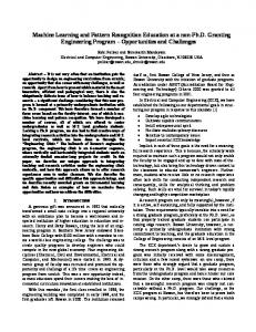
Figure 2: For each output point, extract a neighboring window of data the same size as the facies template. Capture the local dip spectra of the facies template and data window with simple nonstationary “steering filters”. Treating the facies template as the “noise” model, apply a predictive signal/noise separation technique to extract energy from the data window where the local dip coincides with that of the template. The output, simply the noise-to-signal ratio, is then a valid measure of local similarity. morgan2-algorithm2 [NR]
where the operators N and S represent t x domain convolution with prediction-error filters (PEF’s) which decorrelate the unknown noise n and signal s, respectively, and the factor balances the energies of the residuals. Explicitly minimizing the quadratic objective function suggested by equation (3) leads to the following expression for the predicted signal: NT N NT N
s
2 T
S S
1
d
(4)
Since the frequency response of the PEF approximates the inverse spectrum of the data used to estimate it, we see that Abma’s approach is similar to Wiener reconstruction. If the noise is assumed a priori to be spatially uncorrelated, as in Abma (1995), the noise decorrelator N is simply the identity. Gaussian noise is in the nullspace of the PEF estimation, so the signal decorrelator S can be estimated reliably from the data, i.e., S D, where D is a data decorrelating filter. Otherwise, if the noise is correlated spatially, an explicit noise model is required to estimate N, and an approach like the one used by Spitz (1999) to estimate S. Modifying equation (3) to reflect Spitz’s choice of S DN 1 and applying the constraint n d s gives Ns 1
DN s
Nd 0.
(5)
When solved iteratively, the problem can be preconditioned to improve convergence. Following Fomel et al. (1997), we can make the change of variables s
(DN 1 ) 1 p
ND 1 p
(6)
180
Brown & Clapp
SEP–102
and rewrite equation (5): NND 1 p p
Nd 0.
(7)
Brown et al. (1999) solved equation (7) iteratively to suppress ground roll with complicated moveout patterns, where S and N are nonstationary t x-domain PEF’s. Clapp and Brown (1999) did the same for multiple reflections. Unfortunately, the estimation of nonstationary PEF’s is computationally costly, and it is often difficult to ensure that the filters are minimum-phase, a necessary requirement for stable deconvolution, as in equation (7). For the application at hand, the final result is not the estimated signal and noise, but simply the noise-to-signal ratio. It follows that the separation need not be perfect - just good enough to distinguish between regions of the data with gross similarity to the facies template from the rest of the data. A properly stacked or migrated seismic image should have no “crossing dips,” and so can be conceptualized as a single-valued spatial function of local dip angle. Not surprisingly, we have found that simple three-point “steering filters” (Clapp et al., 1997), work well for the noise and data decorrelating filters, N and D, required to solve equation (7). The only thing needed to set up the steering filters is an estimate of the local dip field of the data and facies template, for which the automatic dip scanning technique of Claerbout (1992) produces satisfactory results. Assuming that a given 2-D wavefield u(t, x) is planar with unknown local dip p, the operator p (8) x t will extinguish it. If x and t are finite difference stencils for the continuous partial derivatives above, then equation (8) can be rewritten as a convolution, and hence cast as a univariate optimization for p: r ( x p t ) u(t, x) 0. (9) Differentiating the quadratic functional r T r with respect to p gives an optimal estimate of the local dip: xu tu p (10) tu tu RESULTS Synthetic Data Test Figure 3 shows the synthetic seismic dataset and associated local dip estimate. Figure 4 shows the facies templates used to test the algorithm and their corresponding local dip estimates. The seismic data is a 200x100 2-D slice of the “quarter dome” 3-D model used to test seismic coherency algorithms (Claerbout, 1998; Schwab, 1998), and is characterized by two unconformities. The facies templates, 30x30 points each, are designed to resemble the upper and
SEP–102
Seismic pattern recognition
181
Figure 3: Left: Synthetic data, a modification of the “quarter-dome” model. Right: Estimated local dip. morgan2-syn-datshow [ER]
Figure 4: Top: Facies templates, corresponding to the upper and lower unconformities in the data (Figure ??), respectively. Bottom: Estimated local dip of facies templates shown above. morgan2-syn-trnshow [ER]
182
Brown & Clapp
SEP–102
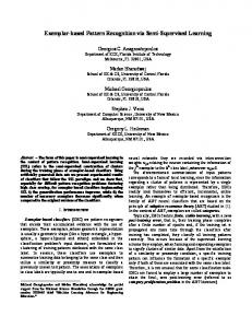
lower unconformities, respectively, but are not windowed directly from the data itself. Notice that the dip changes continuously across the faces of the unconformities. Figures 5 and 6 show the output of the pattern recognition program, where the experiments were designed to detect the upper and lower unconformities, respectively. The results are good, but expected, given the high quality of the estimated dip, and provide adequate proof of concept.
Figure 5: Left: Synthetic data. Center: Output similarity attribute, relative to upper unconformity. Right: Local data windows corresponding to the 98th percentile and higher values in the similarity attribute. morgan2-syn-pmatch2 [ER]
Real Data Test Figure 7 shows the real 2-D seismic image and its associated local dip estimate. The image processed here is a 200x200 subwindow from a migrated 2-D section originally acquired by Mobil over a Gulf of Mexico prospect. The upper portion of the windowed data is characterized by an unconformity. Figure 8 shows the facies template used to test the algorithm and the corresponding local dip estimate. The 50x50 template was created artificially and is designed to resemble the unconformity in the data. The quality of the dip estimates is critical to the success of the algorithm, but unfortunately these estimates are more prone to error with real data than they are for synthetic data (Compare Figures 3 and 7). In order to maximize the spatial coherency of the input data, and hence the robustness of the dip estimate, some smoothing of the data may be required prior to processing. In this case, the estimated dip field was smoothed using a local weighted mean filter, where the weights are the so-called “normalized correlation” measure of Claerbout (1992) - roughly speaking, a measure of the data’s local “plane-waveness”. Figure 9 shows the output of the pattern recognition program. The results are good, having effectively done the same job as a human interpreter, even with a less-than-perfect dip estimate (Figure 8).
SEP–102
Seismic pattern recognition
183
Figure 6: Left: Synthetic data. Center: Output similarity attribute, relative to lower unconformity. Right: Local data windows corresponding to the 98th percentile and higher values in the similarity attribute. morgan2-syn2-pmatch2 [ER]
Figure 7: Left: Sub-window from real 2-D seismic image. Right: Estimated local dip. morgan2-seis-datshow [ER]
Figure 8: Left: Facies templates, corresponding to the unconformities in the upper part of the data (Figure 7). Right: Estimated local dip. morgan2-seis-trnshow [ER]
184
Brown & Clapp
SEP–102
Figure 9: Left: Window from real 2-D seismic image. Center: Output similarity attribute, relative to lower unconformity. Right: Local data windows corresponding to the 98th percentile and higher values in the similarity attribute. morgan2-seis-pmatch2 [ER]
DISCUSSION Given quality local dip estimates of the facies template and seismic image, our approach may seem like overkill. The simplest alternative would be a direct subtraction approach, i.e., extract small windows the same size as the facies template from the seismic image’s dip estimate, then take the RMS difference of it and the facies template’s dip estimate and sum to get the attribute value. Such an approach would surely suffer from the extreme sensitivity of Claerbout’s (1992) dip estimation technique to discontinuities in the data. The estimated local dip is anomalously high at discontinuities, and would thus skew a sum of squared differences. Bednar (1997) defined the dip estimate as a coherency attribute based on this property. A second alternative method might use the fact that any decorrelating filter whitens the spectrum of the data. If a decorrelating filter is obtained for the facies template, then convolved with the seismic image, the local spectrum of the output should be whitest where the image most resembles the facies template. Unfortunately, this would require some measure of whiteness, i.e., how closely does the local autocorrelation of the residual resemble a spike, so in some sense we’d be back to square one. In any case, the authors have found through experience that direct interpretation of the residual to this end is often nonintuitive. In practice, the method will interpret some regions which are obviously not the same geologic feature as the facies template as such. This brings up an important caveat: the program interprets data in terms of local dip spectrum only; not contextually. Such contextual interpretation is best done by a human, and certainly this will remain true for some time. Our method simply makes human interpretation of 3-D images feasible by directing the interpreter to the
SEP–102
Seismic pattern recognition
185
regions of the data which have a local dip spectrum which might match the facies template. Look for regions in Figure 9 which have a similar dip spectrum as the template of Figure 8 – you should be able to find many. The algorithm we presented is still in prototype stage, but nontheless, we are encouraged by the performance characteristics. The algorithm required approximately five minutes on a single processor of our SGI Origin 200 to compute the real data example (Figure 9), including the dip estimation. We subsampled the 200x100-point output space by a factor of five, both spatially and temporally, for a total of 1600. These figures are not stunningly good, considering that the number of output points in many 3-D seismic images may number a million or more, but two facts leave room for improvement. First, since the output depends only on the input, the algorithm is highly parallelizable. Second, since the actual signal/noise separation panels are not output, we have found that the number of iterations per output point may be cut radically, say to five or less. Our approach may also be useful in AVO analysis. AVO anomalies are relatively easy to spot, meaning a simple facies template, but the sheer volume of the data makes hand interpretation tedious. Currently our approach operates on 2-D data only, and we believe that the extension to 3-D is possible, but there are theoretical issues to take stock of. Fomel (1999) discusses these issues in detail; I paraphrase his work here. In 2-D, the dip p is a scalar value; in 3-D it is a T vector: p px p y . Plane waves in 3-D can be extinguished (Schwab, 1998) by a cascade of convolutional operators similar to the operator of equation (8). The matrix equivalent of such an operator is nonsquare and thus noninvertible. Unfortunately, for this application, we require the inverse, i.e., equation (7) Dubbing this composite operator A, Fomel forms AT A and performs spectral factorization to produce a single minimum phase operator.
REFERENCES Abma, R., 1995, Least-squares separation of signal and noise with multidimensional filters: Ph.D. thesis, Stanford University. Bednar, J. B., 1997, Least squares dip and coherency attributes: SEP–95, 219–225. Brown, M., Clapp, R. G., and Marfurt, K., 1999, Predictive signal/noise separation of groundroll-contaminated data: SEP–102, 111–128. Castleman, K. R., 1996, Digital image processing: Prentice-Hall. Claerbout, J. F., 1992, Earth Soundings Analysis: Processing versus Inversion: Blackwell. Claerbout, J. Geophysical Estimation by Example: Environmental soundings image enhancement:. http://sepwww.stanford.edu/sep/prof/, 1998. Clapp, R. G., and Brown, M., 1999, Applying sep’s latest tricks to the multiple suppression problem: SEP–102, 91–100.
186
Brown & Clapp
SEP–102
Clapp, R. G., Fomel, S., and Claerbout, J., 1997, Solution steering with space-variant filters: SEP–95, 27–42. Fomel, S., Clapp, R., and Claerbout, J., 1997, Missing data interpolation by recursive filter preconditioning: SEP–95, 15–25. Fomel, S., 1999, Plane wave prediction in 3-d: SEP–102, 101–110. Leon-Garcia, A., 1994, Probability and random processes for electrical engineering: AddisonWesley. Randen, T., Reymond, B., Sjulstad, H. I., and Soenneland, L., 1998, New seismic attributes for automated stratigraphic facies boundary detection: New seismic attributes for automated stratigraphic facies boundary detection:, 68th Annual Internat. Mtg., Soc. Expl. Geophys., Expanded Abstracts, 628–631. Schwab, M., 1998, Enhancement of discontinuities in seismic 3-D images using a Java estimation library: Ph.D. thesis, Stanford University. Spitz, S., 1999, Pattern recognition, spatial predictability, and subtraction of multiple events: The Leading Edge, 18, no. 1, 55–58.
252
SEP–102