Hindawi Publishing Corporation Journal of Applied Mathematics Volume 2013, Article ID 590614, 18 pages http://dx.doi.org/10.1155/2013/590614
Research Article Selecting Optimal Feature Set in High-Dimensional Data by Swarm Search Simon Fong,1 Yan Zhuang,1 Rui Tang,1 Xin-She Yang,2 and Suash Deb3 1
Department of Computer and Information Science, University of Macau, Macau Faculty of Science and Technology, Middlesex University, UK 3 Department of Computer Science and Engineering, Cambridge Institute of Technology, Ranchi, India 2
Correspondence should be addressed to Simon Fong;
[email protected] Received 22 July 2013; Revised 1 October 2013; Accepted 8 October 2013 Academic Editor: Zong Woo Geem Copyright © 2013 Simon Fong et al. This is an open access article distributed under the Creative Commons Attribution License, which permits unrestricted use, distribution, and reproduction in any medium, provided the original work is properly cited. Selecting the right set of features from data of high dimensionality for inducing an accurate classification model is a tough computational challenge. It is almost a NP-hard problem as the combinations of features escalate exponentially as the number of features increases. Unfortunately in data mining, as well as other engineering applications and bioinformatics, some data are described by a long array of features. Many feature subset selection algorithms have been proposed in the past, but not all of them are effective. Since it takes seemingly forever to use brute force in exhaustively trying every possible combination of features, stochastic optimization may be a solution. In this paper, we propose a new feature selection scheme called Swarm Search to find an optimal feature set by using metaheuristics. The advantage of Swarm Search is its flexibility in integrating any classifier into its fitness function and plugging in any metaheuristic algorithm to facilitate heuristic search. Simulation experiments are carried out by testing the Swarm Search over some high-dimensional datasets, with different classification algorithms and various metaheuristic algorithms. The comparative experiment results show that Swarm Search is able to attain relatively low error rates in classification without shrinking the size of the feature subset to its minimum.
1. Introduction With the advances of information technology, it is not uncommon nowadays that data that are stored in database are structured by a wide range of attributes, with the descriptive attributes in columns and instances in rows. Often among the attributes, a column is taken as a target class. Therefore a classifier can be built by training it to recognize the relation between the target class and the rest of the attributes, with all the samples from the instances. This task is generally known as supervised learning or model training in classification. The model is induced by the values of attributes which are known as features because each one of these contributes to the generalization of the model with respective to its dimension of information. For example, in the wine dataset [1] which is a popular sample used for benchmarking classification algorithms in machine learning community, thirteen attributes (features) of chemical analysis are being used to determine the origin
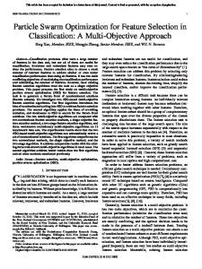
of wines. Each one of these features is describing the origin of the wines which is the target class, pertaining to their respective constituents found in each of the three types of wines. The features essentially are the results of a chemical analysis of wines grown in the same region in Italy but derived from three different cultivars. The features include variables of alcohol content, malic acid level, magnesium, flavonoids, phenols, proline, and color intensity. The multiple features essentially give rise to thirteen different dimensions of influences. In mutual consideration of these influences, a classifier is able to tell the type of wine when it is subject to an unknown sample (which again is described by these thirteen attributes). The multidimensions of these features are visualized in Figure 1. It can be seen that classification is a matter of computing the relations of these variables in a hyperspace to the respective classes; and of course the computation gets complicated as the amount of feature grows. In machine learning, feature selection or input selection is often deployed to choose the most influential features
2
Journal of Applied Mathematics Attribute 1
Class Classes
3
2 1
0
200
14
4
3
12
2
2
10
0 0
0
100
200
0
2 0
100
200
100
0
0
200
0
100
200
200
1
200
10
0
4
0.5
2 0
100
200
Attribute 9
1
0
100
200
0
0
100
200
Attribute 13
1000
2 100
100
2000
3
0
0
Attribute 12 4
1 0
1
20
Attribute 8
4
Attribute 11
5
200
Attribute 4 30
Attribute 7
2
10
100
0
6
Attribute 10 Classes
200
2
15
0
100 Attribute 6
100 50
4
4
150
Attribute 3
6
Attribute 5
200
Classes
100
Attribute 2
16
0
100
200
0
0
100
200
Figure 1: Visualization of multidimensions of features that describe the types of wine.
(inputs) from the original feature set for better classification performance. Feature selection is to find an optimal feature subset from a problem domain while improving classification accuracy in representing the original features. It can be perceived as an optimization process that searches for a subset of features which ideally is sufficient and appropriate to retain their representative power describes the target concept from the original set of features in a given data set. Through the process of feature selection, dimensions in the data are reduced, and the following advantages can be potentially attained: accuracy of the classifier is enhanced; resource consumption is lowered, both in computation and memory storage; it is easier for human to cognitively understand the causal relationship between features and classes with only few significant features. In general, there is no best method known so far that can be unanimously agreed on among data mining researchers in implementing the optimum feature selection. Due to the nonlinear relations of the features and the concept targets, sometimes removing an attribute which has little correlation with the target variable (but unknowingly it is an important factor in other composite dependencies with the other attributes) may lead to worse performance. Tracing along the nonlinearity of the relation for evaluating the worthiness of the attributes is an exhaustive search in the high-dimensional space. Heuristics are often used to overcome the complexity of exhaustive search. In the literature, many papers have reported on the use of heuristics to tackle the feature selection problems. However it is noticed by the authors that many proposed methods are limited to one or more of the following constraints in their designs. See Table 1 for details. (1) The size of the resultant feature set is assumed to be fixed. Users are required to explicitly specify the maximum dimension as the upper bound of the feature set. Though this would significantly cut
down the search time, the search is confined to only the combinations of feature subsets in the same dimensions. Assume that there is a maximum of 𝑘 features in the original dataset. There are 2𝑘 possible combinations of arranging the features in a subset of any variable size. With a bound 𝑠 (for all 𝑠 ≥ 1) imposed on the size of the feature subset, it becomes a combinational problem of picking exactly 𝑠 features into the subset from a total of 𝑘 features. The number of combinations reduces from 2𝑘 to 𝑘!/(𝑘 − 𝑠)!𝑠!. The major drawback is that users may not know in advance what would be the ideal size of 𝑠. (2) The feature becomes minimal. By the principle of removing redundancy, the feature set may shrink to its most minimal size. Features are usually ranked by evaluating their worthiness with respective to the predictive power of the classifier, and then eliminating those from the bottom of the ranked list. Again, there is no universal rule on how many features ought to be removed. Users may have to arbitrarily define a threshold value above which the ranked features form a feature set. (3) The feature selection methods are custom designed for some particular classifier and optimizer. An optimizer is referred to some heuristics that explore the search space looking for the right feature set. As reported in most of the papers in the literature, a specific pair of classifier and optimizer is formulated out of many possible choices of algorithms. The limitations above gave impetuses to the objective of research paper. We opt to design a flexible metaheuristic called Swarm Search that can efficiently find an optimal group of features from the search space; at the same time, there is no need for the user to fix the feature set size as Swarm Search would provide an optimal length of the feature set as well.
Journal of Applied Mathematics
3 Table 1: A brief survey on feature selection models.
Reference Talbi et al. [2] Vieira et al. [3] Wang et al. [4] Abd-Alsabour and Moneim [5] Casado et al. [6] Jona and Nagaveni [7] Unler et al. [8] Korycinski et al. [9] Yusta [10] Unler and Murat [11] Garc´ıa-Torres et al. [12] El Ferchichi and Laabidi [13] Al-Ani [14]
Classifier SVM SVM RS SVM DA SVM SVM BHC N/A LR NB SVM ANN
Metaheuristic PSO, GA BPSO, GA SS ACO TS ACO, Cuckoo PSO TS GRASP, TS, MA PSO, SS, TS TS TS, GA ACO
No. of features N/A 12, 28 14, 15 17–70 54–121 78 10–267 242 18–57 8–93 9–70 24 40, 50
Fixed subset size N/A No No No Yes (5–8) Yes (5) Min Yes (3–8) Yes (3–7) Yes (3–8) No No No
Domain Gene microarray SEPSIS data Credit scoring General General Mammogram General Hyperspectral General General General Urban transport Speech, image
Legends: Particle swarm optimization (PSO), genetic algorithm (GA), support vector machines (SVM), binary particle swarm optimization (BPSO), scatter search (SS), rough set (RS), ant colony optimization (ACO), tubu search (TS), discriminant analysis (DA), binary hierarchical classifier (BHC), memetic algorithm (ma), greedy randomized adaptive search (GRASP), logistic regression (LR) classifier: naive Bayes (NB), Classifier, and Artificial neural network (ANN).
The mechanism of Swarm Search is universal in a sense that different classifiers and optimizers can just plug and play. As a comparative study, several popular classification algorithms coupled with several different most recent metaheuristic methods are integrated into Swarm Search in turn; their performances are evaluated over a collection of datasets of various multitudes of features. In essence the contribution of the paper is a Swarm Search feature selection method which can find optimal features as well as feature set size. The remaining paper is structured as follow. Some related feature selection methods are reviewed in Section 2. The Swarm Search method is described in detail in Section 3. Comparative experiments and their results are presented and discussed in Section 4. Section 5 at the end concludes the paper.
2. Related Work In the past decades, many methods of feature selection have been proposed and studied extensively [15]. In general, there are three types of feature selection designs at the operation level and two types of feature searches at the data exploration level. The three different operational designs are filter-based, wrapper-based, and embedded-based. Often features are evaluated individually in filter-based feature selection model. Features that are found redundant by means of some statistical computation are eliminated. Classification model that adopts filter-based approach evaluates and selects the features during the preprocessing step but ignores the learning algorithm. Hence the aspect of predictive strength of the classifier resulted from different combinations of features is not taken in account during the selection. These are simple selection procedures based on statistical criteria that can be found in a number of commercial data mining software programs. It was pointed out [16] that such methods are not very efficient; especially, when the data carry features,
the maximum accuracy is rarely attained. Some typical measure criteria include information gain [17, 18] mutual information like redundancy relevance and class conditional interaction information, for measuring net relevance of features. Another classical filter method is correlation-based filter method (CFS) from [19] where correlation is used as selection criterion. CFS uses a scoring mechanism to rate and include those features that are highly correlated to the class attribute but have low correlation to each other. However, all the filter-based methods are considering relations among individual attributes and/or between pairs of attributes and target classes. The main drawback of this filter-type method is that it ignores the effect of the subset of features in the induction algorithm, as claimed in [20]. The other type of model is called wrapper-based model, which is popularly on par with the filter-type but generally yields better performance. Wrapper-based method works in conjunction with the induction algorithm using a wrapper approach [20]. The wrapper-based model selects features by considering every possible subset of them; the subsets of features are ranked according to their predictive power, while treating the inbuilt classifier as a black box. An improved version of wrapped-based model is proposed in [21]. It considers information of relevance and redundancy of the features in addition to their influences on the predictive power. The last type is embedded model, which in contrast to wrapper approaches, selects features while taking into account the classifier design [22]. This type is relatively rare for it involves specialized software design in order to enable its dual. Its popularity is hampered due to the complexity of the coding and implementation. It is apparent that exhaustive search under all the wrapper-based and perhaps embedded approaches can be performed, if the number of feature is not too large. However, the problem is known to be NP-hard (Nondeterministic Polynomial Time), and the search quickly becomes computationally intractable. This is especially true for wrapper-based
4
Journal of Applied Mathematics
Classifier
Dataset
Training set Feature selector Raw data
Model induction
Optimizer
Error rate Yes Satistifed?
Optimal subset of features
No Testing set
Classification testing
Heuristic search
Performance evaluation Candidate subset of features
Figure 2: Process model of the proposed swarm search.
models that do rely on a classifier to determine whether a feature subset is good or not. The classifier is being induced continually as the model tries out a new feature subset in a vast search space. The repetition of classifier induction surely incurs high computational costs when the search of feature subsets is brute-force. In order to alleviate the problem of intensive computation, metaheuristic search instead of brute-force search is augmented with certain classifiers in the wrapper-based models. Therefore, an optimal (reasonably good) solution is obtained in lieu of deterministic solution which may take forever to discover. In the literature, a number of contributions belong to this category of hybrid models. Not meant to be exhaustive, Table 1 lists some works in which metaheuristic algorithms are used together with classifiers, in a wrapper approach. In common they are proposed to be targeted at solving the high-dimensionality problems in feature selection by searching for optimal feature subset stochastically. However, some of the works assume that a user-input threshold value is used for defining the size of the feature subset, which was already mentioned as one of the disadvantages in Section 1. Comparing to the earlier research in the 80s and 90s where mostly feature selection belonged to the filter-type focusing mainly on the pairwise relations between the features and the targets recent advances trend towards using wrapper methods to guide the feature selection based on the direct predictive influences by an augmented classifier. Different metaheuristics are used to generate an optimal solution. However, most of the works concentrate on a single type of classifier as well as one or a few specific metaheuristics only. As it can be seen from Table 1, the amount of original features that were being verified by their models in experiment, limit from 8 to 267, except may be the work [2] on microarray. These relatively small feature numbers may not be sufficiently for stress-testing the performance of the proposed algorithms. Lastly but importantly, the model designs in quite a number of works [6, 7, 9–11] are constrained by the need of inputting a pre-defined value for the length of the resultant feature subset; [8], on the other hand, programmed the selection to produce the least amount of features in a feature subset. Often the globally optimal solution, that yields the highest classification accuracy or
other performance criterion by the fitness function, resides in feature subsets beyond this specific predefined subset length. Given these shortcomings as observed from the literature review, it inspires to design an improved feature selection model that is flexible so that different classifiers and metaheuristic optimizer can be easily and compatibly interchanged; the optimal feature subset would be sought on the fly without the need of setting an arbitrary subset length and putting the model under tougher tests of more features (hence higher dimensionality).
3. Proposed Model 3.1. System Work Flow. The design of our model is wrapperbased that consists of two main components—classifier and optimizer as shown in Figure 2. Each of these components can be installed with the corresponding choice of algorithm at the user’s will. Generically, a classifier can embrace software codes of SVM, ANN, decision tree, and so forth. optimizer can be implemented by any metaheuristic algorithm which searches for the optimal feature subset in the highdimensional search space. Over the original dataset which is formatted by all the original features vertically and the full set of instances horizontally, the feature selector module retrieves and cuts the data as per requested by the classifier module and optimizer module. The optimizer module signals the feature selector with the requested features, as resulted from its latest search. The feature selector then harvests the required data of only those feature columns and sends them to the classifier. The classifier uses a 10-fold cross validation method for dividing the corresponding dataset chosen by the feature selector, for training and testing a classifier model (in memory). Classification performance results such as accuracy % and/or other measures could be used as the fitness to the fitness function. In this case, the quality of the classifier model is regarded as the fitness function. As usual a convergence threshold can be set, so that if the fitness value falls below the threshold which is the stopping criterion, the iteration of the stochastic search would stop. Overall, we can see that the process model of our proposed Swarm Search is comprised of two phases. In
Journal of Applied Mathematics the first phase, which is called feature subset exploration and selection, the optimizer searches for the next best feature subset according to the logics of the metaheuristic algorithm installed at the optimizer module which selects the best subset. At the first run, the feature subset would be chosen randomly. In the second phase, which is called learning and testing, at the classifier module, a classifier model is induced from the training data, that is partitioned by feature selector with the best feature subset, and is tested on the test data. The two phases are repeated continually until some stopping criterion is reached, either the maximum number of runs is reached or the accuracy of the classifier is assessed to be satisfactory. In each repetition, the relative usefulness of the chosen subset of features is evaluated and supposedly will improve in comparison to that of the previous round. The classifier here is taken as a black box evaluator, informing how useful each chosen subset of features is by its accuracy. This wrapper approach by default could be brute-force by starting with the first feature subset and tests on all other possible subsets until the very last subset. Obviously this involves massive computation time, or even intractable. For only 100 features, there are 2100 ≈ 1.2677 × 1030 possible subsets for the classifier model to be repeatedly built and rebuilt upon. This high computation costs may further intensify if the training data has many instances. In this regard, we propose to use coarse search strategies like those described in Section 3.1 for the Swarm Search model. Instead of testing on every possible feature subset, the Swarm Search which is enabled by multiple search agents who work in parallel would be able to find the most currently optimal feature subset at any time. It was however pointed out by Yang [23] that there is no free lunch in achieving the optimal feature subset. The feature subset may be the best so far the search has been outreached in the search space, but the absolute global best solution will not be known until all have been tried which may never occur because of the computational infeasibility. 3.2. Swarm Search. A flexible metaheuristic called Swarm Search (SS) is formulated for feature selection by combining any swarm-based search method and classification algorithm. Given the original feature set of size 𝑘, 𝐴 = {𝑎1 , 𝑎2 , . . . , 𝑎𝑘 }, SS supports constructing a classifier with classification accuracy rate 𝑒 by providing an optimal feature subset 𝑆 ∈ 𝐴 such that 𝑒(𝐴) ≥ 𝑒(𝑆), where 𝑆 is one of all the possible subsets that exist in the hyperspace of 𝐴. The core of SS is the metaheuristic algorithm that scrutinizes the search space for an optimal feature subset. Three metaheuristics are used in the experiments in this paper. They are particle swarm optimization (PSO), bat algorithm (BAT), and wolf search algorithm (WSA). 3.2.1. Metaheuristics Algorithms. PSO is inspired by the swarm behaviour such as fish, birds, and bees schooling in nature. The original version was developed by Kennedy and Eberhart in 1995 [24]. The term called Swarm Intelligence was coined since PSO became popular. The dual movement of a swarming particle is defined by its social sense and its
5 own cognitive sense. Each particle is attracted towards the position of the currently global best 𝑔∗ and its own locally best position 𝑙𝑖∗ in history. While at the same time with the effect of the attraction, it has a tendency of moving randomly. Let 𝑙𝑖 and V𝑖 be the location vector and velocity for particle 𝑖, respectively. The new velocity and location and location updating formulas are determined by V𝑖𝑡+1 = V𝑖𝑡 + 𝛼𝜀1 [𝑔∗ − 𝑙𝑖𝑡 ] + 𝛽𝜀2 [𝑙𝑖∗ − 𝑙𝑖𝑡 ] , 𝑙𝑖𝑡+1 = 𝑙𝑖𝑡 + V𝑖𝑡+1 ,
(1)
where 𝜀1 and 𝜀2 are two random vectors, and each entry taking the values between 0 and 1. The parameters 𝛼 and 𝛽 are the learning parameters or acceleration constants, which can typically be taken as [25], 𝛼 ≈ 𝛽 ≈ 2. BAT is a relatively new metaheuristic, developed by Yang in 2010 [25]. It was inspired by the echolocation behaviour of microbats. Microbats use a type of sonar, called echolocation, to detect prey, avoid obstacles, and locate their roosting crevices in the dark. These bats emit a very loud sound pulse and listen for the echo that bounces back from the surrounding objects. Their pulses vary in properties and can be correlated with their hunting strategies, depending on the species. Most bats use short, frequency-modulated signals to sweep through about an octave, while others more often use constant-frequency signals for echolocation. Their signal bandwidth varies depending on the species and often increases by using more harmonics. Three generalized rules govern the operation of the bat algorithm, and they are as follow. (1) All bats use echolocation to sense distance, and they also know the difference between food/prey and background barriers by instinct. (2) Bats fly randomly with velocity V𝑖 at position 𝑥𝑖 with a fixed frequency 𝑓min , varying wavelength 𝜆, and loudness 𝐴 0 to search for prey. They can automatically adjust the wavelength of their emitted pulses and adjust the rate of pulse emission 𝑟 ∈ [0, 1], depending on the proximity of their target. (3) Although the loudness can vary in many ways, we assume that the loudness varies from a large and positive 𝐴 0 to a minimum constant value 𝐴 min . The new solution 𝑥𝑖𝑡 and velocities V𝑖𝑡 at time step 𝑡 are given by 𝑓𝑖 = 𝑓min + (𝑓max − 𝑓min ) 𝛽, V𝑖𝑡 = V𝑖𝑡−1 + (𝑥𝑖𝑡 − 𝑥∗ ) 𝑓𝑖 ,
(2)
𝑥𝑖𝑡 = 𝑥𝑖𝑡−1 + V𝑖𝑡 , where 𝛽 ∈ [0, 1] is a random vector drawn from a uniform distribution. Here 𝑥∗ is the current global best location which is located after comparing all the solutions among all the 𝑛 bats. As the product 𝜆 𝑖 𝑓𝑖 is the velocity increment, we can use either 𝑓𝑖 or 𝜆 𝑖 to adjust the velocity change while fixing
6
Journal of Applied Mathematics
the other factor. Initially, each bat is randomly assigned a frequency which is drawn uniformly from [𝑓min , 𝑓max ]. For local search, once a solution is selected among the current best solutions, a new solution for each bat is generated locally using random walk 𝑥new = 𝑥old + 𝜀𝐴𝑡 ,
(3)
where 𝜀 ∈ [−1, 1] is a random number, while 𝐴𝑡 = ⟨𝐴𝑡𝑖 ⟩ is the average loudness of all the bats at this time step. The update of the velocities and positions of bats have some similarity to the procedure in the PSO as 𝑓𝑖 essentially controls the pace and range of the movement of the swarming particles. The loudness and rate of pulse emission have to be updated accordingly as the iterations proceed. As the loudness decreases once, a bit has found its prey, while the rate of pulse emission increases. Consider = 𝛼𝐴𝑡𝑖 , 𝐴𝑡+1 𝑖 𝐴𝑡𝑖 → 0,
𝑟𝑖𝑡+1 = 𝑟𝑖0 [1 − exp (−𝛾𝑡)] , 𝑟𝑖𝑡 → 𝑟𝑖0 ,
as 𝑡 → ∞.
(4)
WSA [26] is one of the latest metaheuristic algorithms by the authors; its design is based on wolves’ hunting behavior. Three simplified rules that govern the logics of WSA are presented as follow. (1) Each wolf has a fixed visual area with a radius defined by V for 𝑋 as a set of continuous possible solutions. In 2D, the coverage would simply be the area of a circle by the radius V. In hyperplane, where multiple attributes dominate, the distance would be estimated by the Minkowski distance, such that 𝑛
1/𝜆
𝜆 V ≤ 𝑑 (𝑥𝑖 , 𝑥𝑐 ) = ( ∑ 𝑥𝑖,𝑘 − 𝑥𝑐,𝑘 ) 𝑘=1
,
𝑥𝑐 ∈ 𝑋,
(5)
where 𝑥𝑖 is the current position, 𝑥𝑐 are all the potential neighboring positions near 𝑥𝑖 and the absolute distance between the two positions must be equal to or less than V, and 𝜆 is the order of the hyperspace. For discrete solutions, an enumerated list of the neighboring positions would be approximated. Each wolf can only sense companions who appear within its visual circle, and the step distance by which the wolf moves at a time is usually smaller than its visual distance. (2) The result or the fitness of the objective function represents the quality of the wolf ’s current position. The wolf always tries to move to better terrain, but rather than choosing the best terrain it opts to move to better terrain that already houses a companion. If there is more than one better position occupied by its peers, the wolf will chose the best terrain inhabited by another wolf from the given options. Otherwise, the wolf will continue to move randomly in Brownian motion. The distance between the current wolf ’s location and its companion’s location is considered. The greater
this distance is, the less attractive the new location becomes, despite the fact that it might be better. This decrease in the wolf ’s willingness to move obeys the inverse square law. Therefore, we get a basic formula of betterment: (𝑟) =
𝐼𝑜 , 𝑟2
(6)
where 𝐼𝑜 is the origin of food (the ultimate incentive) and 𝑟 is the distance between the food or the new terrain and the wolf. It is added with the absorption coefficient, such that using the Gaussian equation, the incentive formula is 2
𝛽 (𝑟) = 𝛽𝑜 𝑒−𝑟 ,
(7)
where 𝛽𝑜 equals 𝐼𝑜 . (3) At some point, it is possible that the wolf will sense an enemy. The wolf will then escape to a random position far from the threat and beyond its visual range. The movement is implemented using the following formula: 2
𝑥 (𝑖) = 𝑥 (𝑖) + 𝛽𝑜 𝑒−𝑟 (𝑥 (𝑗) − 𝑥 (𝑖)) + escape () ,
(8)
where escape() is a function that calculates a random position to jump to with a constraint of minimum length, V, 𝑥 is the wolf which represents a candidate solution, and 𝑥(𝑗) is the peer with a better position as represented by the value of the fitness function. The second term of the above equation represents the change in value or gain achieved by progressing to the new position. 𝑟 is the distance between the wolf and its peer with the better location. Step size must be less than the visual distance. Given these rules, we summarize the WSA in pseudocode as in Algorithm 1. 3.2.2. Searching for Optimal Feature Subsets. Each search agent in the metaheuristic (PSO/BAT/WSA) is coded as a solution vector which contains a list of feature indices that form a feature subset. The length of a solution vector is variable and it represents the length of the feature subset. At initialization, the vector length is randomized for each search agent. So they have different lengths to start with, in a way similar to placing the search agents in random dimensions of the search space. Each search agent has a variable 𝑘, which is the current length of feature subset it represents, where 1 ≤ 𝑘 ≤ 𝐾. 𝐾 is a constant that is the maximum cardinality of the search space that is also the maximum number of the original features. During the Swarm Search, the search agent steps in the same dimension in each local step movement. The agent explores feature subsets in same dimension. It will only change its dimension at exceptional events. The exceptional events are similar in context to the escape function in WSA, mutation in GA, where a search agent suddenly deviates largely from its local search area (dimension). The exceptional events are usually programmed to happen randomly with
Journal of Applied Mathematics
7
Objective function f(x), x = (x1 , x2 ,. . .,xd )T Initialize the population of wolves, x i (i = 1, 2, . . ., W) Define and initialize parameters: r = radius of the visual range s = step size by which a wolf moves at a time 𝛼 = velocity factor of wolf p a = a user-defined threshold [0..1], determines how frequently an enemy appears WHILE (t < generations && stopping criteria not met) FOR i = 1 : W // for each wolf Prey new food initiatively(); Generate new location(); // check whether the next location suggested by the random number generator is new. If not, repeat generating random location. IF (dist(xi , xj ) < r && x j is better as f(xi ) < f(xj )) x i moves towards x j // x j is a better than x i ELSE IF x i = Prey new food passively(); END IF Generate new location(); IF (rand ()> pa) x i = x i + rand () + v; // escape to a new pos. END IF END FOR END WHILE Algorithm 1: Pseudocode for the WSA algorithm.
a user-defined probability. At the occurrence of such events, the 𝑘 variable changes randomly to other value. In other words, the search agent “jumps” out of its local proximity to another dimension of the search space. For example, an agent has the current dimension 𝑘 = 4; in the next iteration 𝑘 may change to 5, 9785 or any other dimension when an exceptional event occurs. Or else, it would remain the same dimension and explore other combinatorial subsets in the same dimension. The vector of a search agent with 𝑘 = 4 may take a sample form ⟨1, 2, 5, 8⟩ that means that the vector consists of the 1st, 2nd, 5th, and 8th features as the representative indices. A sample snapshot of a search agent exploring the search space and its possible moves is shown in Figure 3. In our design, search agents normally explore in the same dimension in each movement. This is shown as the grey arrows for the case of WSA, hunting for food (looking for a feature subset that produces higher accuracy) randomly in the same dimension. In this way, it only can achieve a local optimal in the same dimension. Because the agents have the tendency to swarm towards their neighbour that have a better fitness function, an active agent (𝑎1 , 𝑎3 ) may merge to its peer agent (𝑎1 , 𝑎3 , 𝑎4 ) provided that the peer agent is having a better fitness. At times, a dimension change function gets activated by the randomizer; the active agent, for example, may “jump” out of its dimensions to another dimension. The random function rand() is a standard Matlab function which produces uniformly distributed pseudorandom numbers. Another random function is to compute about how far the dimension displacement can take, with the direction of (+/−) randomly generated too. The length of jump, however, cannot exceed
beyond the boundary. For instance, the active search agent is now at (𝑎1 , 𝑎3 ), it cannot fall beyond dimension 1. Likewise it can never go beyond the maximum dimension 𝐾. The operation of the optimizer called Swarm Search takes the following steps. (1) Initialize search agents. For each search agent, randomly assign a different feature combination as a subset. (2) Calculate the fitness of the objective function for each agent, rank the agents by their fitness values, and record the one that has the highest fitness as the most promising solution. (3) Perform local search and optimize the current best solution. This step may vary slightly for different metaheuristic algorithms. However, generaly, it tries to update the promising solution unless some satisfactory terminal condition is met. In PSO, the swarming particles have velocities. So we need not only to update their positions, but also to update their velocities. Recording the best local solution and global solution in each generation is required. In BAT, for each generation, rank the current best position according to the pulse rate and loudness; then update the velocity and position for each agent. In WSA, each search agent is updated by three intermediate procedures: first randomly move to update the position; second, check if they are ready to swarm towards to the closest and best companions; third, activate the escape function at random-relocate agents that are qualified to jump dimensions.
8
Journal of Applied Mathematics (a1 , a2 , a3 , a4 ) Escape
Escape
(a1 , a2 , a3 )
(a1 , a2 , a4 )
Active (a1 , a2 )
Peer
Merge
(a1 , a3 )
Prey
Prey
(a2 , a3 , a4 )
(a2 , a3 )
(a2 , a4 )
(a3 , a4 )
(a1 , a4 )
Escape
Prey (a2 )
(a1 )
(a1 , a3 , a4 )
(a3 )
(a4 )
Figure 3: An illustration of possible moves of a search agent in the search space. Table 2: List of feature selection methods used in experiments. Method abbreviation FS-PSO-PN FS-PSO-DT FS-PSO-NB FS-BAT-PN FS-BAT-DT FS-BAT-NB FS-WSA-PN FS-WSA-DT FS-WSA-NB FS-Cfs-PN FS-Cfs-DT FS-Cfs-NB
Classifier Pattern Network Decision Tree Na¨ıve Bayes Pattern Network Decision Tree Na¨ıve Bayes Pattern Network Decision Tree Na¨ıve Bayes Pattern Network Decision Tree Na¨ıve Bayes
(4) Change dimension randomly. (5) Check if the terminating criteria are met; if not go back to step (2). (6) Terminate and output the result.
4. Experiment The Swarm Search feature selection is designed for achieving the following merits (1) low error rate for the classifier as a feature selection tool to harvest the optimal feature subset out from a prohibitively large number of subsets; (2) reasonable time for the convergence of the metaheuristic search when compared to brute-force exhaustive search (whose timetaken we can safely assume to be extremely long); (3) an optimal size of feature subset that leads to optimal accuracy for the particular classifier; and (4) its universality in working across different classifiers and metaheuristic optimizers. Concerning the proposed four merits, experiments by computer simulation are then carried out accordingly. We target to evaluate the performance with respect to the first three virtues: (i) average error rate which is simply the number of incorrectly classified instances divided by the total number of testing instances; (ii) the total time consumed in finding the optimal feature subset including the training and testing
Metaheuristic Particle swarm optimization Particle swarm optimization Particle swarm optimization Bat algorithm Bat algorithm Bat algorithm Wolf search algorithm Wolf search algorithm Wolf search algorithm Correlated-based filter Correlated-based filter Correlated-based filter
Approach Swarm Swarm Swarm Swarm Swarm Swarm Semiswarm Semiswarm Semiswarm Filter Filter Filter
of the respective classifier, in unit of seconds; and (iii) the length of the feature subset as the percentage of the maximum dimension of the original features. In order to validate the universality of the proposed Swarm Search model, three popular classification algorithms have been chosen to be the kernels of the Classifier, and three contemporary metaheuristic methods are utilized as the core optimizer to perform the Swarm Search exploration. Furthermore, we use an industrial standard feature selection method called correlation-based filter selection (Cfs) for as a baseline benchmark for comparing with the proposed methods. Total there are twelve different feature selection methods that are programmed and tested in our experiments; see Table 2. The classification algorithms as mentioned in Table 2 have been defined and studied in [27]. For the metaheuristic methods, readers who want to have the full details are referred to [24] for PSO, [25] for BAT, and [26] for WSA. Both PSO and BAT have substantial swarming behaviour for their movements that are governed with velocity; a single leader who has the greatest attractiveness is among the agents the remaining agents follow the leader’s major direction, while at the same time they roam locally. In contrast, the agents in WSA are autonomous; they do merge nevertheless only when they come in contact with their visual range. So
Journal of Applied Mathematics
9 Table 3: Datasets that are used in feature selection experiments.
Dataset
Attributes
Instances
Abstract/URL
Lung Cancer
56
32
Heart Disease
75
303
The data refers to the presence of heart disease in the patient
Libra Movement
91
360
The data refers to hand movement type in LIBRAS, Brazilian signal language
Hill Valley
101
606
Either a Hill (a “bump” in the terrain) or a Valley (a “dip” in the terrain)
The data described 3 types of pathological lung cancers http://archive.ics.uci.edu/ml/datasets/Lung+Cancer http://archive.ics.uci.edu/ml/datasets/Heart+Disease http://archive.ics.uci.edu/ml/datasets/Libras+Movement http://archive.ics.uci.edu/ml/datasets/Hill-Valley
CNAE-9
875
1080
Nine categories of free text business descriptions of Brazilian companies http://archive.ics.uci.edu/ml/datasets/CNAE-9
their approach is type of semiswarm. Cfs [19] evaluates the worth of a subset of attributes by considering the individual predictive ability of each feature along with the degree of redundancy between them. Subsets of features that are highly correlated with the class while having low intercorrelation are preferred. The operation of Cfs is filter-based and sequential, hence no swarm. 4.1. Experimental Data and Setup. The twelve feature selection methods with combinations of different classifiers and optimizers are put under test across five well-known dataset from UC Irvine Machine Learning Repository (short for UCI). UCI is popular data archive for benchmarking the performance of machine learning algorithms. The five datasets that are chosen contain various numbers of features, ranging from 56 to 875. They are Lung Cancer, Heart Disease, Libra Movement, Hill Valley, and CNAE-9. Details of these datasets are outlined in Table 3. In addition to a variety of attribute numbers for stress testing the feature selection algorithms, the five datasets are chosen with purposes. Lung cancer is solely a categorical classification problem, where all predictive attributes are nominal, taking on integer values 0–3. The data described 3 types of pathological lung cancers. However this dataset is having relatively few instances available for model training in respective to attributes, with the ratio of attributes-to-instances 56 : 32. It represents a tough disproportional problem in training an accurate classification model. The dataset Heart Disease represents a mixed multivariate data-type problem. Libra Movement dataset represents a challenging hand movement recognition problem, where the data attributes are coordinates, solely numeric, and the data are in sequential order as they were extracted from video frames. Similarly, Hill Valley is a purely numeric and sequential time-series. Sampling at regular intervals over the 𝑥-axis, a variable value fluctuates on 𝑦axis over time. An accurate prediction model for recognizing whether the sequential points are forming a hill or valley is known to be hard to build in the context of pattern recognition with a single sequential variable. CNAE-9 is extremely challenging, because of the large number of attributes that resulted from the word frequency counts. The words and their
combinations that appear in each document may have subtle relations to the nature of the document. All these five chosen datasets present different levels and perspectives of challenges in constructing an accurate classification model and hence in testing the efficacy of each feature selection algorithm. The main performance indicator in the experiments is classification error rate which is also used as stop criterion. The Swarm Search is programmed to explore and rank the solution continually until the difference of the average error rate of the current iteration and that of the recorded best are less than 1.0 × 10⁻⁸ . The other criterion is the maximum iteration which is set arbitrarily at 100,000,000 cycles. The maximum run cycle is to prevent the Swarm Search from running exceedingly long. The dataset, CNAE-9 with the greatest amount of features 875, potentially has 875 dimensions in the search space, and this amounts to 2875 (≈ 2.519 × 𝑒+263 ) combinatorial feature subsets. This enormously large number obviously prevents any normal computer from an exhaustive search. Even using Swarm Search, it will take a very long time indeed, while a deterministic solution is not guaranteed. For the optimizer, default parameter settings are adopted for the metaheuristic methods; the default values are shown in Table 4. We have to be very careful in choosing the parameters as they are sensitive to performance. For different metaheuristic methods, the parameters vary. In BAT, the bat position is influenced by the bat’s echo loudness and echo pulse rate, so adjusting the loudness and emitted pulse depends on the proximity of their target. Here, we use 0.5 as their values, which shall result in a balance of intensification and exploration. The PSO has two learning factors, 𝑐1 , 𝑐2 . Generally, 𝑐1 = 𝑐2 and the value is smaller than 2 as this has been widely used in the literature. In our experiment, we use 1.5 which is moderately less than 2. For WSA, each search agent has a visual circle and the visual distance is the visual radius. In WSA, there is an escape function that simulates how a wolf runs far away from the current position when danger is encountered. The jump over is assumed farther than its visual radius. In our experiment, we set 5 as the escape distance that is five times larger than
10
Journal of Applied Mathematics Table 4: Parameter settings for metaheuristic methods.
FS using BA Parameter A (loudness) R (pulse rate) Populations 𝑄min 𝑄max
value 0.5 0.5 5 0 0.2
FS using PSO Parameter Populations 𝑐1 𝑐2
FS using WSA Parameter Visual distance Escape distance Escape probability Population
value 5 1.5 1.5
value 1 5 0.25 5
Table 5: Comparative results in classification error for all the classification algorithms with Cfs feature selection and swarm search feature selection and without any feature selection. Algorithm PN DT NB Cfs-PN Cfs-DT Cfs-NB PSO-PN PSO-DT PSO-NB BAT-PN BAT-DT BAT-NB WSA-PN WSA-DT WSA-NB
Lung Cancer (56) 0.5938 0.5 0.375 0.3125 0.3438 0.2813 0.125 0.225 0.1513 0.1188 0.21 0.1625 0.1338 0.0407 0.1575
Heart Disease (75) 0.4653 0.4719 0.4422 0.462 0.4818 0.4224 0 0 0.105 0 0 0.27 0 0 0
the visual range. In addition, the escape probability is the probability of encountering danger. For a fair comparison, each metaheuristic method has 5 searching agents which are supposed to run in parallel. They are however programmed to run in sequential on a normal computer (instead of a parallel computer); the five agents move stochastically in round robin under the optimization loop. The programs are coded in Matlab R2010b. The computing environment is a MacBook Pro (with CPU: 2.3 GHZ, RAM: 4 GB). 4.2. Experimental Results. The experiments are mainly grouped into three kinds, testing for the performance of feature selection in classification error, in time consumption, and in amount of features obtained in the feature subset. For classification errors, Table 5 tabulates the results for classifiers using algorithms of Pattern Network (PN), which is also known as Artificial Neural Network, Decision Tree (DT), and na¨ıve Bayes (NB), as well as the results that produced with their feature selection counterparts. Around the five different datasets, the results pertaining to classification errors, are plotted in radar charts visually in Figures 4, 5, and 6, respectively. Likewise, the results for consumption time are in Table 6 and Figures 7, 8, and 9. Table 7 and Figures 10, 11, and 12 are for feature amount in feature subgroup. Please note that for clarify in radar charts, the feature amounts are normalized to percentage with respect to the original feature
Libra Movement (91) 0.1944 0.3028 0.3722 0.1972 0.2583 0.3528 0.075 0.2806 0 0.0833 0.3444 0.1028 0.0694 0.2028 0
Hill Valley (101) 0.4447 0.505 0.5149 0.5017 0.4951 0.4884 0.3465 0.2112 0.0495 0.1997 0.2442 0.5132 0.1997 0.2178 0.1151
Lung cancer (56) 0.35 0.3 0.25 0.2 0.15 0.1 0.05 0
CNAE (875)
CNAE (875) 0.8741 0.112 0.0685 0.187 0.1889 0.1824 0.0083 0.0407 0.8889 0.037 0.0491 0.8889 0.037 0.037 0.8889
Classification error Classifer: pattern network
Heart disease (75)
Libra movement (91)
Hill valley (101) PSO BAT WSA
Figure 4: Results in classification error for Pattern Network are shown visually in radar chart.
numbers when charted. While the tabulated results allow comparison between swarm search and no swarm search at easy glance, the radar charts show individually the efficacy of
Journal of Applied Mathematics
11
Table 6: Comparative results in time consumption (in seconds) for all the classification algorithms with Cfs feature selection and swarm search feature selection and without any feature selection. Algorithm PN DT NB Cfs-PN Cfs-DT Cfs-NB PSO-PN PSO-DT PSO-NB BAT-PN BAT-DT BAT-NB WSA-PN WSA-DT WSA-NB
Lung Cancer (56) 3.07 0.02 ≈0 0.18 ≈0 ≈0 853.23123 177.3407 22.9799 1532.321 179.1062 25.8876 1521.8085 1521.8085 42.2628
Heart Disease (75) 2.35 0.08 0.01 ≈0 0.01 1.26 382.3217 11.9377 3.92775 347.0041 16.5652 2.436514 1305.6519 49.2341 23.3551
Libra Movement (91) 18.08 0.32 0.05 3.79 0.04 0.02 1714.34495 232.6246 82.7123 686.557 240.737 28.6922 3005.4028 106.6606 404.6113
Hill Valley (101) 58.73 0.16 0.08 0.3 ≈0 ≈0 921.28525 491.7232 34.344 524.367 448.7332 31.001802 1159.367 176.6559 24.7167
CNAE (875) 5066.72 3.39 0.26 10.51 0.08 ≈0 70538.3472 2886.9232 2358.2769 26365.1231 2341.6668 1441.7241 26365.1231 82688.1231 236365.123
Table 7: Comparative results in feature amount in feature subgroup for all the classification algorithms with Cfs feature selection and swarm search feature selection and without any feature selection. Algorithm PN/DT/NB Cfs-PN/DT/NB PSO-PN PSO-DT PSO-NB BAT-PN BAT-DT BAT-NB WSA-PN WSA-DT WSA-NB
Lung Cancer (56) 56 11 41 39 37 41 29 38 41 41 35
Heart Disease (75) 75 9 21 44 18 17 50 5 21 23 19
each swarm search variant with respect to the five datasets in visual comparisons. 4.3. Result Analysis. The classification error rates vary a lot across different datasets and with different classifiers. For instance, perfect accuracy is achieved for Heart Disease dataset with all three different optimizers and three different classifiers, except PSO-NB and BAT-NB where their accuracies are 89.5% and 73%, respectively. Moderate error rates are observed for Lung Cancer dataset, but relatively high error rate is incurred on the remaining datasets like Libra Movement, Hill Valley, and CNAE. In one extreme case, for CNAE dataset, Na¨ıve Bayes classifier suffers at almost 89% error rate in all situations of optimizers, but over the same CNAE dataset, classifiers of Pattern Network and Decision Tree can achieve very low error rate less than 5%. This extreme performance is shown in Figure 6. As CNAE represents the worst case of highest dimensionality, Pattern Network classifier managed to conquer the problem of high dimensionality quite well especially with PSO optimizer
Libra Movement (91) 91 26 75 66 19 39 79 6 45 40 20
Hill Valley (101) 101 1 96 79 9 88 84 43 30 44 82
CNAE (875) 875 28 853 854 76 849 781 243 849 851 323
(less than 1% error); See Figure 4. It works quite well with BAT and WSA too (at 3.7% error) considering that the dataset is text mining in nature and there are many variables for determining the category of documents that the text would belong to. Na¨ıve Bayes apparently is rated down upon this CNAE dataset. However, it works well for the rest except Hill Valley which is basically time-series dataset with 101 data points forming a shape of hill or valley. The hills and valleys in the time series form nonlinear recursion which is postnonlinear combination of predecessors. The classifier needs to recognize the shape by processing the values of the data points. The mathematical challenge is due to the problem of post-nonlinear multidimensional data projection. Na¨ıve Bayes did not do well with Bat but otherwise with PSO (