Suppression by Selecting Wavelets for Feature Compression in

1

Suppression by Selecting Wavelets for Feature Compression in Distributed Speech Recognition Syu-Siang Wang, IEEE student member, Payton Lin, Yu Tsao, Jeih-Weih Hung, and Borching Su, IEEE members

Abstract—Distributed speech recognition (DSR) splits the processing of data between a mobile device and a network server. In the front-end, features are extracted and compressed to transmit over a wireless channel to a back-end server, where the incoming stream is received and reconstructed for recognition tasks. In this paper, we propose a feature compression algorithm termed suppression by selecting wavelets (SSW) for DSR: minimizing memory and device requirements while also maintaining or even improving the recognition performance. The SSW approach first applies the discrete wavelet transform (DWT) to filter the incoming speech feature sequence into two temporal subsequences at the client terminal. Feature compression is achieved by keeping the low (modulation) frequency sub-sequence while discarding the high frequency counterpart. The low-frequency sub-sequence is then transmitted across the remote network for specific feature statistics normalization. Wavelets are favorable for resolving the temporal properties of the feature sequence, and the down-sampling process in DWT reduces the amount of data at the terminal prior to transmission across the network, which can be interpreted as data compression. Once the compressed features have arrived at the server, the feature sequence can be enhanced by statistics normalization, reconstructed with inverse DWT, and compensated with a simple post filter to alleviate any over-smoothing effects from the compression stage. Results on a standard robustness task (Aurora-4) and on a Mandarin Chinese news corpus (MATBN) showed SSW outperforms conventional noise-robustness techniques while also providing nearly a 50% compression rate during the transmission stage of DSR systems. Index Terms—discrete wavelet transform, feature compression, distributed speech recognition, data transmission efficiency.

I. INTRODUCTION PEECH recognition is an essential component of the user interface. As mobile devices become smaller, distributed speech recognition (DSR) has become increasingly important since complex recognition tasks are often difficult to perform due to restrictions in computing power, access speed, memory capacity, and battery energy [1]–[3]. To handle these resource limitations, packet-based DSR systems utilize a client-server architecture [4]–[7] and follow the European Telecommunications Standards Institute (ETSI) standard [8], which defines the standard feature extraction and compression algorithms to reduce the transmission bandwidth. The front-end is responsible for extracting and compressing the speech features prior to transmitting over a wireless channel. In the back-end, the features are recovered for decoding and recognition on a powerful server. Conducting speech feature compression on the mobile device only requires a small portion of the overall computation and storage, and can improve data channels by reducing bandwidth and frame-rates. However, performance of even the best current stochastic recognizers degrades in

S

unexpected environments. Therefore, designing a compact representation of speech that contains the most discriminative information for pattern recognition while also reducing computational complexity has been a challenge. In addition, with upcoming applications that aim to combine speech with even more diverse features from multimodal inputs [9]–[12], determining a practical compression scheme remains a priority. Briefly speaking, there are two main goals for DSR systems: selecting a representation that is robust while also improving the data transmission efficiency. For the first goal, articulatory features incorporate the events and dynamics [13], while filter-bank (FBANK) [14], Mel-frequency cepstral coefficients (MFCCs) [15], extendedleast-square-based robust complex analysis [16], and power normalized cepstral coefficients (PNCC) [17] are designed to allow the suppression of insignificant variability in the higherfrequency regions. Qualcomm-ICSI-OGI (QIO) features [18] are extracted based on spectral and temporal processing with data compression for client-server systems. Most features are generated by converting the signal into a stream of vectors with a fixed frame rate [19]. These initial features can generally exhibit high discriminating capabilities in quiet settings, however enviromental mismatches caused by background noise, channel distortions, and speaker variations can degrade the performance [20]. Therefore, noise compensation methods are commonly used to produce more robust representations on either normalizing the distributions of a feature stream [13], [21] or extracting speech-dominant components at specific modulation frequencies [22], [23]. Approaches that regulate the statistical moments, which are the expected value of a random variable to any specified power corresponding to the long-term temporal feature sequence, including mean subtraction (MS) [24], mean and variance normalization (MVN) [25], histogram equalization (HEQ) [26], and higher order cepstral moment normalization (HOCMN) [27]. Approaches that filter the time trajectories of the features to emphasize the slowly time-varying components and to reduce spectral coloration include RelAtive SpecTrA (RASTA) [28], MVN plus autoregression moving average filtering (MVA) [29], and temporal structure normalization (TSN) [30]. Approaches that alleviate the noise effects in the modulation spectrum include spectral histogram equalization (SHE) [31], modulation spectrum control (MSC) [32], and modulation spectrum replacement (MSR) [33]. For the secondary goal of the DSR front-end to efficiently forward the data to the remote network, source coding techniques reduce the number of bits during transmission over bandwidth-limited channels and have benefitted real-time

2

voice response services [34]. Approaches based on vector quantization (VQ) [35], [36] split each feature vector on the client side into sub-vectors to quantize via a specified codebook, and include split VQ (SVQ) [37], [38], Gaussian mixture model-based block quantization [34], and histogrambased quantization [39]. Approaches based on variable frame rates [40], [41] select frames according to the speech signal characteristics in order to decrease the number of frames required to represent each front-end feature prior to transmission to back-end recognizers. For example, the Euclidean distance can be calculated between the neighbouring frames of the current frame to determine whether to preserve or discard the frame if the measure is smaller than a weighted threshold [42]–[44]. Methods for threshold derivation include a posteriori signal-to-noise ratio (SNR) weighted energy [45] and an energy weighted cepstral distance [46]. In this study, we propose a novel algorithm applied in DSR to approach the two aforementioned goals, viz. robustness to noise and high data compression. This novel algorithm, named suppression by selecting wavelets with a short-hand notation “SSW”, creates the compressed speech feature that contains the low temporal modulation frequency portion. To be more precise, the compression in SSW does not count on a codebook, but is rather in line with the findings in literature [23], [47]–[49]. [23] reveals that speech components are dominant at low temporal modulation frequencies of the signal, which are also referred to as the dynamic envelopes of acoustic-frequency subbands. Specifically, it has been shown in [47] that most of the useful linguistic information at in the temporal modulation frequencies between 1 Hz and 16 Hz, with the dominant component at around 4 Hz. Also, according to [48], a bandpass modulation filtering that captures lowfrequency spectral and temporal modulations of the acoustic spectrogram for speech signals gives rise to noise-robust speech features, in which the temporal modulations are in the range of 0.5 − 21 Hz. In [49], the data-driven temporal filters for MFCC feature streams to improve noise robustness are also found to be bandpass and emphasize the component at low temporal modulation frequencies. SSW expands our previous studies [50], [51] that normalize the statistics of subband features on discrete wavelet transform (DWT), and is shown to be suitable for deep neural network (DNN) systems [52]–[57]. Wavelets are commonly used in signal and image compression to provide high resolution time-frequency analysis [58]–[62], and are favorable for resolving the temporal properties of speech because they use a sliding analysis window function that dilates or contracts when analyzing either the fast transients or slowly varying phenomena. The first step of SSW applies DWT to decompose the full-band input feature stream into low-modulation frequency component (LFC), and highmodulation frequency component (HFC). The second step of SSW discards the HFC information and only preserves the LFC information prior to transmitting across a network to a remote server. The operation of completely discarding HFC expands previous researches [23], [28] on smoothing the interframe variations to enhance the robustness of features for backend recognizers in the server side while performing feature compression simultaneously by only considering LFC to ad-

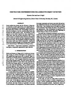
dress both issues of a DSR system. As soon as the LFC feature sequence is received on the server side, the third step of SSW normalizes the LFC sequence to alleviate the environmental mismatch between training and testing phases as in [50], [63]. Next, a feature vector with all-zero elements is prepared as the HFC, which works together with the normalized LFC to reconstruct the new feature stream via inverse DWT (IDWT). The reconstructed feature stream is further compensated via a post high-pass filter, which aims to alleviate possible oversmoothing effects. The resulting features are then used for speech recognition. The SSW approach will be evaluated for DSR using the standard Aurora-4 robustness task [64], [65] and a Mandarin Chinese broadcast news corpus (MATBN) [66]. The hidden Markov model toolkit (HTK) [67] and the Kaldi speech recognition toolkit (Kaldi) [68] will be used to compare recognition performance for SSW versus the baselines of MFCC, FBANK, QIO, MS, MVN, MVA, TSN and RASTA. The experiments in this paper reveals that SSW can accomplish the main goals of DSR: improving performance on the back-end server while also providing up to a 50% compression rate (by discarding the HFC information) during the transmission stage. The rest of this paper is organized as follows: Section II introduces DWT theory and the conventional filtering-based and normalization approaches. Section III covers the steps of the proposed SSW approach. Section IV describes the setups of the DSR systems for Aurora-4 and MATBN and discusses the experimental results and justification. Section V concludes. II. R ELATED A LGORITHMS A. Wavelet transform Figs. 1 and 2 show the flowcharts for one-level DWT and IDWT. The signals being decomposed and reconstructed are denoted as a0 [n] and a ˜0 [n]. The LFC and HFC containing the low-frequency (approximation) and high-frequency (detail) components of a0 [n] are denoted as a1 [n] and d1 [n]. The impulse responses of low-pass and high-pass filter sets for ˜ DWT and IDWT are denoted as {g[n], g˜[n]} and {h[n], h[n]}. Here, the “↓ 2” and “↑ 2” symbols represent the factor-2 downsampling and up-sampling operations. Stating in more detail, Fig. 1 shows the DWT decomposition process and includes the steps of filtering and down-sampling. First, the signal a0 [n] is filtered by g[n] and h[n], and the resulting outputs are individually passed through the factor2 down-sampling operation to create a1 [n] and d1 [n]. Due to down-sampling, the length of a1 [n] and d1 [n] is approximately half the length of the original a0 [n]. The IDWT reconstruction process is shown in Fig. 2 and includes the steps of upsampling, filtering, and addition. First, a factor-2 up-sampling process is conducted on a1 [n] and d1 [n]. Second, the low- and ˜ are separately applied to the uphigh-pass filters g˜[n] and h[n] sampled version of a1 [n] and d1 [n]. Finally, the two filtered signals are added to generate the signal a ˜[n]. It should be noted that a perfect reconstruction can be achieved (˜ a0 [n] = a0 [n−`] with ` a positive integer) by carefully designing the low-pass ˜ and high-pass filters g[n], h[n], g˜[n] and h[n] for DWT and IDWT. In addition, the (one-side) bandwidth for each of these

ℎ[n]

2 2

2 1 0

0 0.5 1 Normalized frequency (# : rad/sample)

𝑑1 [n]

𝑎0 [n] 𝑔[n]

3

Magnitude

and thus they are half-

𝑎1 [n]

3 2 1 0

0 0.5 1 Normalized frequency (# : rad/sample)

2

2

3 2 1 0

0 0.5 1 Normalized frequency (# : rad/sample)

Fig. 3. Frequency responses of the biorthogonal 3.7 filters that are applied to DWT: (a) low- and (b) high-pass filters in the decomposition process; (c) low- and (d) high-pass filters in the reconstruction process.

𝑔[n] ෤

Fig. 2. Block diagram of the reconstruction process, where ↑ 2 represents the factor-2 up-sampling process.

˜ Fig. 3 shows the frequency response of g[n], h[n], g[n], ˜ and h[n] for a commonly used biorthogonal 3.7 wavelet basis, which will be applied in our SSW technique. The biorthogonal X.Y wavelet basis belongs to the biorthogonal wavelets family [69], in which the biorthogonal properties of these filters is defined in Eq. (1), h˜ g [n], g[n − 2`]i = δ[`], ˜ hh[n], h[n − 2`]i = δ[`],

1

˜ jω ) of (d) Frequency response H(e ˜ jω ) of (c) Frequency response G(e ˜ low-pass filter g˜[n] in the reconstruc- high-pass filter h[n] in the reconstruction process. tion process.

ℎ෨ [n] 𝑎෤ 0 [n]

𝑎1 [n]

2

(a) Frequency response G(ejω ) of (b) Frequency response H(ejω ) of low-pass filter g[n] in the decompo- high-pass filter h[n] in the decomposition process. sition process.

Fig. 1. Block diagram of the decomposition process, where ↓ 2 represents the factor-2 down-sampling process.

𝑑1 [n]

3

0 0 0.5 1 Normalized frequency (# : rad/sample)

Magnitude

π 2,

Magnitude

filters listed above is approximately band filters.

Magnitude

3

(1)

˜ h˜ g [n], h[n − 2`]i = hh[n], g[n − 2`]i = 0, where the δ[`] is the Dirac delta function, and h·i represent the inner production operation. In addition, the indices, X and Y , represent the order of vanishing moments for the two low-pass filters g[n] and g˜[n] for DWT and IDWT, respectively [70]. Here, a low-pass filter ψ[n] (ψ[n] ∈ {g[n], g˜[n]}) with the frequency response Ψ(ejω ) having a vanishing moment K for satisfies the following condition: dk |Ψ(ejω )| = 0 for k = 0, 1, ..., K − 1. (2) dω k ω=π Therefore, the vanishing moment K indicates the rate of decaying to zero at frequency π for the frequency response of the filter. High-order vanishing moment shows high decaying rate and the sharp boundary of a filter in the frequency domain. More details for vanishing moments can be found in [71] and [72]. From Fig. 3, we see that all of the filters are approximately half-band. In addition, the magnitude response of the low-pass analysis filter g[n] is symmetric to that of the high-pass synthe˜ sis filter h[n] about the frequency π2 , and so do the high-pass analysis filter h[n] and the low-pass synthesis filter g˜[n]. That ˜ j(π−ω) )| and |H(ejω )| = |G(e ˜ j(π−ω) )|, is, |G(ejω )| = |H(e jω jω jω jω ˜ ˜ where G(e ), H(e ), G(e ) and H(e ) are the Fourier ˜ transform of g[n], h[n], g˜[n] and h[n], respectively. Such a quadratic mirror property is commonly possessed by the wavelet filter sets.

B. Robust feature extraction This section reviews the temporal filtering and statistics normalization algorithms. Fig. 4 illustrates the temporal domain feature extraction for the filtering or statistics normalization. From the figure, the power spectrum of an input speech waveform is first created through the conventional short-time Fourier transform for feature extraction. Next, pre-defined melfilter banks are carried out to filter the power spectrum and to capture the intra-frame spectral information, and followed by the logarithmic operation to form the FBANK feature. The static MFCC feature is derived as well by further applying discrete cosine transform to FBNAK. The delta and delta-delta MFCC features are then extracted and combined with static MFCC to provide final MFCC features of an utterance. Speech Waveform

Processed Features

Original Features Filter/Normalize Filter/Normalize

Feature Extraction

Filter/Normalize 𝑛, time

𝑛, time

Fig. 4. Block diagram of robust feature extraction via filtering/normalization processing.

1) Filtering algorithms: Most approaches [28], [73] are based on the theory that low-modulation frequencies (except the near-DC part) contain the critical aspects of speech. Let ci [n] denote the original time sequence of an arbitrary feature channel i, where n is the frame time index. A new sequence cˆi [n] obtained from ci [n] via a filtering process can be described by cˆi [n] = GF {ci [n]} = h[n] ⊗ ci [n],

(3)

where h[n] is the impulse response of the applied filter. The associated system function is further denoted as H(z). The temporal filter structures of RASTA and MVA integrate a

4

low-pass filter and a high-pass-like process, which acts like a band-pass filter to alleviate the near-DC distortion and also to suppress the high-frequency components in the modulation domain. RASTA uses a filter with the system function: HRAST A (z) = z 4

0.2 + 0.1z −1 − 0.1z −3 − 0.2z −4 , 1 − 0.98z −1

(4)

MVA normalizes the incoming time series to be zero-mean and unity-variance, prior to passing through an ARMA filter: 1 + z −1 + · · · + z −M , (2M + 1)z −M − z −M −1 − · · · − z −2M (5) where M denotes the order of the filter (M is set to 1 in the later experiments). 2) Normalization algorithms: Most approaches reduce the mismatch between the training and testing conditions by equalizing the specific statistical quantities of an arbitrary temporal feature sequence (in the training and testing sets) to a target value. For instance, MS processes the first-order statistical moment, MVN processes the first- and second-order statistical moments, and HEQ normalizes the entire probability density function (PDF), which amounts to all-order statistical moments. In these approaches, the target statistical quantities are usually obtained from all of the utterances of the training set. HARM A (z) =

III. PROPOSED ALGORITHMS Fig. 5 shows the flowchart for the proposed SSW algorithm. In DSR, SSW is split into the client phase and the sever phase. Client system Input feature sequence ci [n] Server system

All-zeros vector, 𝑐𝐻 ǁ 𝑖 [𝑛]=0

HFC, 𝑐𝐻𝑖 [𝑛]

c෤i [n]

Network

Post filter

(6)

where GDW T {·} denotes the one-level DWT operation. If the Nyquist frequency of the input ci [n] is F Hz, then the frequency ranges of ciL [n] and ciH [n] are roughly [0, F/2] Hz and [F/2, F ] Hz. For example, the value of F equals 50 for the commonly used frame rate of 100 Hz. The LFC ciL [n] and HFC ciH [n] will be handled differently: (1) LFC ciL [n] is directly transmitted to the server end (which decreases the length of the original stream ci [n] in half), (2) HFC ciH [n] is completely discarded. These operations are primarily based on the theory that relatively low temporal modulation-frequency components (roughly between 1 Hz and 16 Hz) contain most of the useful linguistic information, and that temporal filters should de-emphasize the high-modulation frequency portions of speech to reduce the noise effect [28], [47]–[49], [74]. Therefore, it is expected that discarding HFC ciH [n] in ci [n] will not degrade the performance. According to the preceding discussion, only the LFC of the input ci [n] is concerned for the subsequent process while its HFC is totally discarded. Therefore, in practical implementations, we can simply pass ci [n] through the low-pass analysis filter g[n] of DWT, and then proceed with the factor2 downsampling, which is depicted in the upper part of Fig. 5 and can be expressed by X ciL [n] = g[`]ci [2n − `]. (7) `

In other words, the high-pass branch of the one-level DWT can be completely omitted here since it has nothing to do with the signal ciL [n], which is to be transmitted to the server end. B. Server system

LFC, 𝑐𝐿𝑖 [𝑛]

IDWT

{ciL [n], ciH [n]} = GDW T {ci [n]},

Discard

DWT

𝑐′𝑖𝐿 [𝑛] Normalize 𝑐𝐿ǁ 𝑖 [𝑛]

distinctive temporal properties of the original sequence ci [n]. This DWT decomposition is formulated by:

Robust Sequence cොi [n]

Fig. 5. Flowchart of SSW in a client-server DSR system. The “Discard” block refers to the step of discarding HFC, the “Normalize” block refers to the statistics normalization, and the “Post filter” block refers to high-pass filter as in Eq. (12). A vector with all-zeros serves as the HFC on the server end. Thus the transmitted stream is one half the length of the original stream ci [n].

In the bottom row of Fig. 5, we assume that the network channel is error-free (with no quantization error, channel i distortion and packet loss) and thus the received LFC c0 L [n] = i 0i cL [n]. c L [n] is first updated via a statistics normalization algorithm, such as MS or MVN, so that the resulting normalized LFC c˜iL [n] will be more robust than the original LFC ciL [n]. Then, SSW uses a zero sequence as the new HFC to be used in the following IDWT process: c˜iH [n] ≡ 0, for all n,

where c˜iH [n] has the same size of c˜iL [n]. Afterwards, IDWT is applied to merge the two half-band components, c˜iL [n] and c˜iH [n], thereby reconstructing a full-band feature sequence as: c˜i [n] = GIDW T {˜ ciL [n], c˜iH [n]},

A. Client system An I-dimensional speech feature {ci [n]; i = 0, 1, ..., I − 1} (such as MFCC, FBANK, or PNCC) is first extracted from each frame of the recorded signal on the client device, where n is the frame index. A one-level DWT is further applied to the feature sequence ci [n] with respect to any arbitrary channel i to obtain the LFC ciL [n] and HFC ciH [n], which carry the

(8)

(9)

where GIDW T {·} denotes the one-level IDWT operation. It should be noted that the IDWT reconstructed sequence c˜i [n] differs from the original sequence ci [n] in Eq. (6), as c˜i [n] is expected to vary more smoothly in time than ci [n] since the HFC of c˜i [n] has been zeroed out, as in Eq. (8). Analogous to the previous discussions, in practical implementations c˜i [n] can be obtained by directly passed the

5

normalized LFC, c˜iL [n], through the factor-2 up-sampling and the low-pass synthesis filter g˜[n], depicted in the lower part of Fig. 5 and expressed by ( c˜iL [ n2 ], if n = 0, 2, 4, · · · , i c˜L,up [n] = (10) 0, otherwise, and c˜i [n] =

X

g˜[`]˜ ciL,up [n − `].

(11)

Client system

c𝑖 [n]

cො𝑖 [n]

𝑔[n] Server system 𝑔[n] ෤ Post filter 𝑐ǁ 𝑖 [𝑛]

c𝑖𝐿 [n] 2 Network

2 Normalize c෤𝑖𝐿 [n] 𝑐′𝑖𝐿 [𝑛]

Fig. 6. The real-operation system of the SSW approach.

`

That is, only the low-pass branch of the IDWT process is put into effect actually. In practice, the IDWT output c˜i [n] was found to be oversmoothed, so a post filter is applied to c˜i [n] to compensate its high-frequency components: α (12) cˆi [n] = c˜i [n] − c˜i [n − 1], 2 where α is a non-negative constant. As a result, cˆi [n] in Eq. (12) serves as the final output of the SSW algorithm. Please note that setting α = 0.0 causes no filtering on cˆi [n], while a positive α amounts to a high-pass filter performed on cˆi [n]. C. Analysis Some discussions about the presented SSW method are as follows: 1) Qualitative analysis: When ignoring the client-server transmission error and the effect of normalization in the SSW process shown in Fig. 5, the relationship between the two spectra, C i (ejω ) and C˜ i (ejω ), of the input ci [n] and the output c˜i [n] (before the final high-pass post-filtering), respectively, can be expressed by ˜ jω ) C˜ i (ejω ) =0.5C i (ejω )G(ejω )G(e ˜ jω ), + 0.5C i (ej(π−ω) )G(ej(π−ω) )G(e

(13)

˜ jω ) are the frequency response of the where G(ejω ) and G(e two low-pass filters, g[n] and g˜[n]. Please note that on the right-hand side of Eq. (13) the term C i (ej(π−ω) )G(ej(π−ω) ) is the mirror image of C i (ejω )G(ejω ) with respect to the central frequency ω = π2 caused by the factor-2 upsampling. In addition, the high-frequency mirror spectrum C i (ej(π−ω) )G(ej(π−ω) ) can be nearly removed by the sub˜ jω ), and thus sequent low-pass synthesis filter G(e ˜ jω ), C˜ i (ejω ) ≈ 0.5C i (ejω )G(ejω )G(e jω

(14)

given that the anti-aliasing filter G(e ) and anti-imaging filter ˜ jω ) have been well designed. G(e According to the flowchart of real-operation system of the SSW approach shown in Fig. 6, the filters being used include g[n] and g˜[n] only, and in fact these two low-pass filters are not necessarily required to be wavelet bases for DWT and IDWT. However, here we adopt the wavelet filters primarily for two reasons: First, DWT/IDWT has been widely applied as an octave-band analysis/synthesis filter bank with down-sampling/up-sampling that can achieve perfect reconstruction of signals. Given that the temporal series of the clean speech features ci [n] has a nearly negligible higher halfband, processing ci [n] with merely the low-frequency branch

in the concatenation of DWT and IDWT can result in a good approximation of ci [n]. Second, the low-pass filters in some particular wavelets families, such as the biorthogonal wavelets stated in sub-section II-A, are designed to have a symmetric impulse response and are thus linear-phase, indicating that they will not introduce phase distortion to the input series ci [n]. 2) Quantitative analysis: At the outset, we conducted a preliminary evaluation to demonstrate that the speech-dominant component for recognition can be captured by SSW. One clean utterance with the transcript “Acer international corporation of Taiwan shows a machine billed as compatible with the bottom hyphen the hyphen line p.s. slash two model thirty period.” was selected from the Aurora-4 database [65] and then artificially contaminated by any of three additive noises (car, street and train-station) at three signal-to-noise ratio (SNR) levels (5 dB, 10 dB and 15 dB). The resulting ten utterances (one clean and nine noisy utterances) were passed through the system shown in Fig. 7. From this figure, each of the utterances was converted to FBANK feature streams, passed through a one-level DWT to obtain the LFC and HFC sub-streams, and normalized by mean subtraction (MS). The obtained LFC and HFC sub-streams were further scaled by the binary weighting factors {βL , βH |βL , βH ∈ {0, 1}} and then fed into the IDWT to reconstruct the FBANK features. For simplicity, the ultimate ˜ β β , in FBANK features of all channels are denoted by C L H which the subscript “βL βH ” was from the aforementioned binary weighting factors indicating if the FBANK features ˜ 11 is the contain either or both of LFC and HFC. Thus C original (MS-processed) FBANK consisting of both LFC and ˜ 10 and C ˜ 01 refer to the LFC and HFC FBANK HFC, and C features, respectively. In addition, the three FBANK features, ˜ 11 , C ˜ 01 and C ˜ 10 , were fed into the CD-DNN-HMM acoustic C models (detailed descriptions were given in Section IV-A) to produce the corresponding 2030 dimensional bottleneck ˜ 11 , M ˜ 01 and M ˜ 10 . Notably here the features, denoted by M bottleneck features were the output of the used CD-DNNHMM without applying the final softmax function. We believe that the results of bottleneck features more directly indicate the classification properties given specific input feature types. ˜ 11 , C ˜ 10 , C ˜ 01 , M ˜ 11 , M ˜ 10 Next, for each feature type (C ˜ and M01 ), the frames of features in the aforementioned ten sentences labelled as the three phone units, “s”, “sh” and “I”, were collected and then processed by principal component analysis (PCA) for dimension reduction. The resulting twodimensional coefficients of the first two PCA axes for each feature type were depicted in Figs. 8(a)-(f). From these figures, we observe that: • The PCA coefficients for those features with respect

6

Speech signal c𝑖𝐿 [n] FBANK feature extraction

MS

DWT c𝑖𝐻 [n]

MS

Bottleneck feature 𝛽𝐿 c෤𝑖𝐿 [n] MS-based IDWT acoustic model 𝛽𝐻 c෤𝑖𝐻 [n]

Fig. 7. Flowchart of the analysis system. The system is designed to confirm the effectiveness of SSW, where LFC and HFC are dominated by speechrelevant and speech-irrelevant components, respectively.

˜ 11 , C ˜ 10 , M ˜ 11 to the original FBANK and LFC, viz. C ˜ and M10 , reveal clear separations among three different phones, as shown in Figs. 8(a)(b)(d)(e). This somewhat implies that both the FBANK and LFC serve as a good feature for phone classification at both clean and noisy conditions. Also, the partial overlap between the clusters of “s” and “sh” is probably owing to the similar physical articulation of these two phones. In addition, the PCA ˜ 11 and C ˜ 10 are quite close, and so are coefficients for C ˜ 11 and M ˜ 10 , indicating that LFC is highly those for M dominant at FBANK while the remaining HFC is rather insignificant in amount. • Unlike the cases of FBANK and LFC, the three phone ˜ 01 and M ˜ 01 ) clusters for two HFC-related features (C significantly overlap with each other, as revealed in Figs. 8(c)(f). Therefore, the HFC features are shown to contain little discriminating information for classifying the three phones, or they are seriously distorted by noise. Accordingly, the LFC captured by SSW is believed to preserve the prevailing element in FBANK for robust speech recognition, while omitting the HFC part in FBANK just eliminates the irrelevant information and thereby forms a more compact feature. Next, to reveal the effect of the post filter shown in Fig. 6, we conduct SSW (with MS as the statistics normalization algorithm) on the FBANK features of a clean utterance in the Aurora-4 database [65]. Four assignments of the parameter α for the filter as in Eq. (12) are used in SSW, and the power spectral density (PSD) curves of three FBANK features are shown in Fig. 9. From this figure, we first find that SSW causes a significant PSD reduction of FBANK features at the high frequency portion (within around the range [30 Hz, 50 Hz]). In addition, a larger value of α used in the post filter of SSW can further emphasize the speech-dominant band (roughly between 10 Hz and 25 Hz) relative to the highly suppressed low frequency portion (below 4 Hz). These observations indicate that SSW with α > 0 can suppress the unwanted noise component of an utterance at high modulation frequencies as well as enhance the respective speech component. IV. EXPERIMENT RESULTS AND ANALYSES This section presents the experimental setups, demonstrates the evaluation of the SSW algorithm, and discusses the results. A. Experimental setup

In the evaluation experiments, the biorthogonal 3.7 wavelet basis set [69] was selected in the DWT/IDWT process of SSW, which frequency responses were shown in Fig. 3. Two databases, Aurora-4 and MATBAN were used for the evaluation, which details are described as follows. Aurora-4 is a medium vocabulary task [65] acquired from the Wall Street Journal (WSJ) corpus [75] at 8 kHz and 16 kHz sampling rate. 7138 noise-free training utterances were recorded with a primary microphone and were further contaminated to form the multi-training set with or without the secondary channel distortions and any of six different types of additive noise (car, babble, restaurant, street, airport, or station) at 10 to 20 dB SNR. The testing data for clean and noisy scenarios contained 14 different test sets (Sets 1-14) with each set containing 330 utterances. A single microphone was used to record Sets 1-7, and different microphones, which distorted utterances with channel noises, were used to record Sets 8-14. Next, Sets 2-7 and Sets 9-14 were further contaminated by the six additive noise types at SNR levels from 5 to 15 dB. All 14 testing sets were further organized to four testing subsets, A, B, C and D on the order of clean (set 1), noisy (sets 2-7), clean with channel distortion (set 8), and noisy with channel distortion (sets 9-14), respectively. In addition, 330 different utterances were recorded for each testing situation to form the development data. For Aurora-4, two DSR systems were implemented, one based on HTK [67] and the other based on Kaldi [68]. In addition to 39-dimensional MFCCs (including 13 static components plus their first- and second-order time derivatives), and 40-dimensional FBANK features, we implemented 45dimensional QIO as comparative features that were designed to perform data compression for client-server systems [18]. For the HTK system, the training and testing data at 8 kHz sampling rate were used to simulate a more challenging condition. 166 utterances for each test set were selected and used to test recognition as suggested in [65]. The multi-condition training data were used to train the context-dependent (CD) triphone acoustic models, where each triphone was characterized by a hidden Markov model (HMM) with 3 states and 8 Gaussian mixtures per state and 16 mixtures per state was applied to the silence. For the Kaldi system, the training and testing data at 16 kHz sampling rate were used to test performance. All 330 utterances for each test set were applied to test system performances [65]. The clean-condition training data were used to train CD Gaussian mixture model HMM (CD-GMMHMM) based on the maximum likelihood (ML) estimation criterion. With the fixed CD-GMM-HMM, the extracted QIOor FBANK-based robust features were applied to train CDDNN-HMM model. Seven layers were used for the DNN structure. The same structure was used in several previous studies that test recognition performance on Aurora-4 [76], [77]. Among these layers, there were five hidden layers with each layer containing 2048 nodes. The input layer for the DNN had 440 (40 ∗ (5 ∗ 2 + 1)) dimensions for 5 left/right context frames, and the output layers had 2030 nodes. A set of trigram language models was created based on the reference transcription of training utterances. Evaluation results are reported using word error rate (WER).

7

30

30

20

20

10

10

0

0

-10

-10

4

"I" "s" "sh"

2 0

-20

-10

0

10

20

-20

30

˜ 11 (a) The PCA-processed C 200

100

100

0

0

-100

-100

-100

0

100

-10

0

10

20

30

-4 -6

˜ 10 (b) The PCA-processed C

200

-200 -200

-2

-200 -200

˜ 11 (d) The PCA-processed M

100

50

-4

-2

0

2

4 ˜ (c) The PCA-processed C01

6

"I" "s" "sh"

0

-100

0

100

˜ 10 (e) The PCA-processed M

-50

-100

-50

0 ˜ (f) The PCA-processed M01

˜ 11 , (b) C ˜ 10 and (c) C ˜ 01 , and PCA-processed (d) M ˜ 11 (e) M ˜ 10 and (f) M ˜ 01 with respect to “I” (blue dot Fig. 8. Scatter plots of PCA-processed (a) C points), “s” (red circle marks) and “sh” (green cross marks) on clean and nine different noisy conditions.

SSW (α = 0.0) SSW (α = 0.8) SSW (α = 1.6) SSW (α = 2.0)

(Hz) (a) The first dimension

(Hz) (b) The 20-th dimension

(Hz) (c) The 39-th dimension

Fig. 9. PSDs of the (a) first (i = 0) (b) 20-th (i = 19) (c) 39-th (i = 38) dimensional FBANK-feature streams are derived on one clean utterance, which is selected from the training set of Aurora-4. In addition, the original speech feature is also processed by SSW with α = 0, 0.8, 1.6, and 2.0.

MATBN is a 198-hour Mandarin Chinese broadcast news corpus [66], [78], recorded from Public Television Service Foundation of Taiwan that contains material from a news anchor, several field reporters and interviewees. The material was artificially segmented into utterances, and contained background noise, background speech, and background music. A 25-hour gender-balanced subset of the speech utterances was used to train the acoustic models. A 3-hour data subset was used as the development set (1.5 hours) and the testing set (1.5 hours). MATBN was originally recorded at a 44.1 kHz

sampling rate, and further down-sampled to 16 kHz. For MATBN, a DSR system was implemented on the Kaldi [68] toolbox with three types of speech features: 39dimensional MFCCs (including 13 static components plus their first- and second-order time derivatives), 40-dimensional FBANK, and 45-dimensional QIO features. MFCCs with MVN extracted from the training data were selected for training CD-GMM-HMM. With the fixed CD-GMM-HMM, the extracted QIO- or FBANK-based robust features were applied to train CD-DNN-HMM model. DNN structures contained eight layers, with six hidden layers and 2048 nodes per layer.

8

TABLE I T HE VOLUME ( UNIT: M AGA B YTES , MB) OF FBANK AND SSW ( ON PROCESSED -FBANK) FEATURES REQUIRED IN THE SERVER SYSTEMS FOR THE TRAINING DATA IN AURORA -4 AND MATBN, AND THE AVERAGED COMPRESSION RATIO OF EACH UTTERANCE ( DENOTED AS “AVG .”). Database Aurora-4 MATBN

Volume for FBANK 414.89 MB 685.90 MB

Volume for SSW 211.37 MB 361.85 MB

Avg. 48.87% 46.72%

TABLE III E XPERIMENTAL RESULTS FOR MS AND SSW WITH RESPECT TO DIFFERENT α VALUES ON THE DEVELOPMENT SUBSET OF AURORA -4 IN K ALDI - BASED DSR. α

0.0

0.4

0.8

1.2

1.6

2.0

MS

WER

35.05

28.02

27.18

26.83

26.41

27.11

27.80

TABLE II T HE VOLUME ( UNIT: M AGA B YTES , MB) OF FBANK AND SSW ( ON PROCESSED -FBANK) FEATURES REQUIRED DURING TRANSMISSION BY THE CLIENT TO THE SERVER SYSTEMS FOR THE TESTING DATA IN

AURORA -4 AND MATBN, AND THE AVERAGED COMPRESSION RATIO OF EACH UTTERANCE ( DENOTED AS “AVG .”). Database Aurora-4 MATBN

Volume of FBANK 257.55 MB 12.12 MB

Volume of SSW 131.32 MB 6.34 MB

Avg. 48.88% 47.26%

This model structure gave the best performance tested on the development set. The input layer for DNN-HMMs had 440 (40 ∗ (5 ∗ 2 + 1)) dimensions for 5 left/right context frames, and the output layer had 2596 nodes. Evaluation results are reported as the average character error rates (CER). B. Experimental results The results of the Aurora-4 (English) and MATBN (Mandarin) tasks are presented in three perspectives: (1) data compression, (2) recognition results, and (3) qualitative analysis. 1) Data compression: Tables I and II show the volumes of the original and SSW (LFC of FBANK) features for the training data (stored on the server end), and for the testing data (transmitted from the client end). The compression ratio is calculated between the volumes of original features (VO ) and the SSW features (VS ), as defined in Eq. (15). Tables I and II show SSW immediately reducing the stored and transmitted data volume by approximately 50%, which is a result of the factor-2 down-sampling operation of DWT (as well as the discarding operation of the HFC from the original feature sequence). Although these data compression results are significantly large in size, it will be important to determine if these compressed SSW features can actually maintain or even improve the recognition accuracy in DSR applications. VS (15) VO 2) Recognition results: We first conducted experiments to investigate the correlation of the parameter α in SSW with the recognition accuracy. Table III shows the recognition results in terms of WER of the Kaldi-based DSR tested on the development subset of Aurora-4, where this subset was formed by selecting 330 utterances from all of the 14 development sets. The MS result is also reported in Table III for comparison. From the table, lower WERs as compared to MS are noted when α values are larger than 0.8. In addition, when α is 1.6, the SSW yields the lowest WER. Based on the results in Table Ratio = 1 −

Fig. 10. On HTK-based DSR system, performance (WER) for MFCCs, and MFCCs processed by either MVN, MVA, and SSW on subsets A, B, C, and D of Aurora-4.

III, α was set 1.6 to test SSW on Aurora-4 in the Kaldi-based DSR in the following experiments. We also tested recognition using development sets to determine the optimal α in SSW for other DSR systems for both Aurora-4 and MATBN tasks. In the following discussions, we reported the SSW results with the optimal α determined by the development sets. Table IV shows the Aurora-4 results from the HTK-based DSR system for the 14 test sets (Sets 1-14) for MFCC and QIO, as well as MFCCs processed by MS, MVN, MVA, TSN and RASTA. It is clear that MS, MVN, and TSN improved the performance by lowering the WERs when compared to QIO and MFCCs. Moreover, it is noted that MVA outperformed MS, MVN, RASTA and TSN by combining normalization and the low-pass ARMA filter. The results of the proposed SSW algorithm were also reported in the last row of Table IV. For this task, the SSW approach selects MVN to normalize the LFC feature streams (as shown in Fig. 5), and sets the parameter α in Eq. (12) to zero. Table IV shows SSW achieved the lowest average WER, and actually improved the performance on the clean set (Testing Set 1). Fig. 10 shows results of MFCC, MVN, MVA and SSW on four testing subsets A, B, C, and D. From the figure, SSW provided the lowest WERs for subsets A, B, and D, and performed almost as well as MVA for subset C. These results demonstrate the effectiveness of SSW for extracting robust features in HTK-based DSR systems. Table V shows the Aurora-4 results from the Kaldi-based DSR system for the 14 test sets (Sets 1-14) for FBANK and QIO, as well as FBANKs processed by MS, MVN, MVA, TSN, RASTA, and SSW. For this task, the SSW approach selects MS to normalize the LFC feature streams (as shown

9

TABLE IV O N THE HTK- BASED DSR SYSTEM , WER S OF MFCC, QIO, AND MFCC PROCESSED BY FILTERING OR NORMALIZATION APPROACHES ON THE 14 TEST SETS OF THE AURORA -4 TASK . B OLD SCORES DENOTE THE BEST PERFORMANCE . T HE AVERAGE PERFORMANCE IS DENOTED AS AVG . Set

1

2

3

4

5

6

7

8

9

10

11

12

13

14

Avg.

MFCC QIO MS MVN MVA TSN RASTA SSW

10.83 11.20 13.08 11.16 11.16 8.73 13.74 10.64

12.04 10.98 11.79 10.68 10.68 9.21 11.57 10.42

20.04 19.19 17.94 16.32 15.87 13.59 16.65 15.80

22.91 20.74 22.98 20.41 20.81 16.50 22.80 20.55

23.94 19.96 22.28 18.31 19.34 13.22 19.04 18.60

20.04 18.12 19.12 15.73 16.35 12.82 17.02 16.02

24.97 20.81 22.95 19.45 19.26 16.94 20.15 19.15

16.57 13.92 14.59 13.37 12.89 17.31 24.60 13.00

19.37 16.35 15.73 16.13 14.73 18.38 23.46 15.06

26.85 22.14 24.64 22.91 21.77 31.05 31.58 22.17

30.57 26.11 27.51 26.63 26.63 30.50 32.26 26.26

33.66 25.97 29.80 25.82 25.75 32.01 36.10 25.23

27.70 23.68 22.84 23.13 22.62 27.18 32.36 22.65

31.86 25.27 27.48 24.46 25.01 32.97 34.70 24.42

22.95 19.60 20.91 18.89 18.78 20.03 24.00 18.57

TABLE V O N THE K ALDI - BASED DSR SYSTEM , WER S OF FBANK, QIO, AND FBANK PROCESSED BY FILTERING OR NORMALIZATION APPROACHES ON THE 14 TEST SETS OF THE AURORA -4 TASK . B OLD SCORES DENOTE THE BEST PERFORMANCE . T HE AVERAGE PERFORMANCE IS DENOTED AS AVG . Set

1

2

3

4

5

6

7

8

9

10

11

12

13

14

Avg.

FBANK QIO MS MVN MVA TSN RASTA SSW

3.08 3.87 2.95 3.16 3.23 3.31 3.83 2.93

3.87 5.34 3.96 4.15 4.22 4.17 4.35 3.61

6.37 8.99 6.18 6.05 5.98 5.77 7.27 5.27

7.68 10.80 7.02 7.08 7.55 7.49 9.06 6.58

6.93 10.89 6.18 6.54 7.64 6.82 7.15 5.92

5.94 9.10 5.88 5.88 6.28 5.94 7.44 5.10

7.79 9.71 6.03 7.27 7.19 6.37 8.01 6.54

9.04 6.16 6.20 6.07 6.41 5.53 7.70 5.94

12.20 9.47 8.03 8.78 9.43 7.92 9.77 7.92

18.96 15.47 17.80 16.61 18.03 17.47 18.51 15.97

22.70 19.20 17.26 18.96 20.68 19.43 19.73 16.53

22.44 17.11 17.15 17.37 18.61 17.11 18.08 16.31

18.14 15.56 16.27 16.50 16.70 16.12 17.69 13.67

22.06 15.67 18.46 16.87 17.99 16.63 19.93 17.34

11.94 11.24 9.96 10.09 10.71 10.01 11.32 9.26

TABLE VI O N THE K ALDI - BASED DSR SYSTEM , CER S OF FBANK, QIO, AND FBANK PROCESSED BY FILTERING OR NORMALIZATION APPROACHES ON THE MATBN TASK . B OLD SCORES DENOTE THE BEST PERFORMANCE .

CER

FBANK 12.84

QIO 14.96

MS 12.24

MVN 12.04

MVA 12.57

TSN 12.76

RASTA 15.01

SSW 12.04

in Fig. 5), and sets the parameter α in Eq. (12) to 1.6. Table V shows SSW achieved the lowest average WER, and also improved the performance on the clean test (Testing Set 1). These findings were similar to those observed in the HTK system in Table IV. Fig. 11 shows results of FBANK, MVN, MS and SSW on four testing subsets A, B, C, and D. From the figure, SSW provided the lowest WERs for subsets B, C and D, and similar performance as MS for subset A. These results demonstrate the effectiveness of SSW feature compression for extracting robust features for Kaldi-based DSR system. In summary, the results show SSW can handle the issues of additive noise and channel distortions, which were demonstrated in subsets C and D in Figs. 10 and 11, as well as provide better recognition accuracy for both clean and noisy conditions in Aurora-4 relative to the other approaches. When combined with the ability to provide feature compression as shown in Table I and Table II, these findings offer conclusive evidence that the proposed SSW approach achieves the main goals of DSR: minimizing memory and device requirements while also maintaining or even improving the recognition performance.

Fig. 11. On the Kaldi-based DSR system, WERs for FBANK, and FBANK processed by MVN, MVA, and SSW on subsets A, B, C, and D of Aurora-4.

Additional experiments were also conducted using MATBN, which is a more realistic task since the data contains utterances that are of low-quality and intelligibility (with mispronunciations, repairs, and repetitions) and have real-world noises

10

and background speech (unlike the digitally additive noise of Aurora-4). Table VI shows DNN-HMM results for baseline FBANK and QIO, as well as FBANKs processed by either of MS, MVN, MVA, TSN, RASTA and SSW. The results show SSW outperforming MS, MVA, TSN and RASTA, and providing similar performance to MVN. Since SSW also offers data compression as shown in Table I and Table II, these findings offer conclusive evidence that SSW achieves the main goals of DSR: selecting a representation that is robust while also improving the data transmission efficiency. 3) Qualitative analysis: In this section, we present the statistical properties of SSW using the histograms from the entire training and test sets. Figs. 12 and 13 show the histograms on Aurora-4 (MFCC and FBANK), and Fig. 14 shows the feature histograms on MATBN (FBANK). In these figures, the probability density functions (PDF) of the training and test sets are denoted as pT r and pT s . The x-axis and y-axis in all subfigures represent the values and corresponding probabilities of the features. The first, second and third rows of Fig. 12 show the results for the first, 4th and 12th dimensional features while those rows in Fig. 13 and Fig. 14 are the results for the first, 20th and 40th dimensional features. For further comparisons, every subfigure also provides the Kullback-Leibler divergence (KL) score between pT r and pT s as calculated in Eq. (16): X pT s (x) , (16) KL = pT s (x)log p T r (x) x where x is the value in the x-axis. It should be noted that a KL divergence score with a lower value indicates a higher similarity between the two PDFs of pT r and pT s . From Fig. 12, we observe that (1) The histograms of the training and test sets of SSW and MVN matched better when compared to those of MFCC. (2) When compared to MVN, the KL divergences of SSW was notably lower at the first dimension while similar for the other two dimensions. Next, from Fig. 13 and Fig. 14, we observe that (1) The histograms of the training and test sets of SSW matched better when compared to those of FBANK and MS. (2) The KL divergences of SSW were lower when compared to those of FBANK and MS. The above observations indicate that SSW offered high statistical matching between the training and test sets by using the integration of the normalization and filtering operations. These findings provide quantitative supports to explain the promising capability of SSW reported in Tables IV, V, and VI. C. Discussion In the section, we first provide additional experimental results to further illustrate the advantages of the SSW algorithm. Then, we summarize the novelty and contribution of SSW. 1) Combining SSW with PNCC: To further demonstrate the effectiveness of SSW, we implemented the PNCC [17] algorithm, which is a state-of-the-art feature extraction method designed based on the consideration of human auditory system to alleviate the effects of additive noise and room reverberation. In this set of experiments, 39-dimensional PNCC (including 13 static components plus their first- and secondorder time derivatives) were extracted from the utterances of

Aurora-4 and MATBN and further processed by SSW (termed PNCC-SSW) for evaluating on CD-DNN-HMM DSR systems. For Aurora-4, the averaged WERs of PNCC and PNCCSSW over 14 test sets were 11.46% and 11.01%, respectively. On the other hand, the CERs of PNCC and PNCC-SSW in MATBN were 13.77% and 13.76%, respectively. Please note that PNCC-SSW reduces the number of feature frames by half when compared to PNCC. These results demonstrate that SSW can perform well to highlight the linguistic information and noise-robust component in the feature, not only MFCC and FBANK (as reported in the previous section), but also PNCC. 2) In noise-free environments: From Tables IV and V, we observed that the SSW can further improve the performance of clean Testing Set 1. To further demonstrate the performance of SSW in noise-free environments, two more experiments were conducted. First, we constructed HTK-based and Kaldibased DSRs, which used the clean training data at 8 kHz and 16 kHz sampling rates, respectively, in Aurora-4. The training procedure of these two systems was similar to that used in Section IV-A, while the multi-condition training set was not used. For HTK-based DSR, we compared the results of MFCC and SSW, and for Kaldi-based DSR, we compared the results of FBANK and SSW. The clean Testing Set 1 in Aurora-4 was used to the recognition. The WERs for MFCC and SSW in the HTK-based systems were 8.91% and 8.40%, respectively, while the WERs for FBANK and SSW in the Kaldi-based system were 3.06% and 2.78%, respectively. The results confirm again that the proposed SSW algorithm can improve the original features by promoting the recognition accuracy, even both training and testing data were recorded in a noise-free condition. Second, we conducted speech recognition using another test data recorded in a noise-free condition: a subset of WSJ [75] training set, which contained 1516 clean utterances pronounced by ten speakers, recorded at 16 kHz sampling rate. Those data were selected from the set labeled ”si tr s”, and they had no overlap with the training utterances in Aurora4. Here, the acoustic models were the ones that were used to recognize FBANK and SSW features (as reported in Table V). Please note that these two sets of acoustic models were trained using the multi-condition training set. The recognition results in terms of WERs for FBANK and SSW were 31.59% and 22.99%, respectively. These results again show that SSW can give further improvements even under noise-free environments. 3) Bit-wise compression and packet loss: As presented in Section IV-B, the SSW algorithm can reduce the amount of data in a feature-frame-wise compression. In a network transmission scenario, quantization techniques such as pulse code modulation (PCM) [79] and SVQ [80]–[82] for bitwise compression are often performed on speech features to conserve the transmission bandwidth. Briefly speaking, the PCM technique quantizes each element in a feature into the pre-defined 2b level and thus reduces the storage requirement for each element to b bits, and SVQ-based approaches first construct a series of codebooks along the feature dimension using the training set, and then use these codebooks to encode the features in the testing set with a small number of bits

11

SSW Fig. 12. Histograms and KL divergences from the Aurora-4 training and test sets for (a) MFCC, or MFCC processed by either (b) MVN, or (c) SSW. The first, second and third rows indicate the statistical histograms of the first, 4-th and 12-th dimensional feature vectors.

SSW Fig. 13. Histograms and KL divergences from the Aurora-4 training and test sets for (a) FBANK, or FBANK processed by either (b) MS, or (c) SSW. The first, second and third rows indicate the statistical histograms of the first, 20-th and 40-th dimensional feature vectors.

12

0.1000

pTr(x)

0.1000

KL=0.0315

pTs(x)

0.1000

0

pTr(x)

10

20

30

0.0000 -20

0.1000

KL=0.0141

pTs(x)

0.0000 -20

0.1000

-10

0

pTr(x)

10

20

30

-10 pTr(x)

0

10

20

30

KL=0.0131

0.0000 -20

0.1000

20

30

0.0000 -20

0

10

20

30

KL=0.0010

pTs(x) 0.0500

-10 pTr(x)

0

10

20

30

KL=0.0013

0.0000 -20

-10

0

10

pTr(x)

0.1000

20

30

KL=0.0006

pTs(x)

0.0500

0 10 (a) FBANK

-10 pTr(x)

pTs(x)

0.0500

-10

0.0000 -20

0.1000

KL=0.0035

0.0500

pTs(x)

0.0000 -20

0.0500

pTs(x)

0.0500

KL=0.0084

pTs(x)

0.0500

-10

pTr(x)

0.1000

KL=0.0202

pTs(x)

0.0500 0.0000 -20

pTr(x)

0.0500

-10

0 10 (b) MS

20

30

0.0000 -20

-10

0 10 (c) SSW

20

30

Fig. 14. Histograms and KL divergences from the MATBN training and test sets for (a) FBANK, or FBANK processed by either (b) MS, or (c) SSW. The first, second and third rows indicate the statistical histograms of the first, 20-th and 40-th dimensional feature vectors.

before transmitting them through the network. Relative to the original data before encoding and transmitting, the received and decoded data on the server side contain distortions including quantization errors as well as losing packets. In the following, we investigate the effect of the combination of SSW (feature-frame-wise compression) and either of the quantization techniques (bit-wise compression) on the noisy DSR scenario that suffers from packet loss. For integrating SSW with PCM, the client side of DSR first extracted LFC features from FBANK and recorded each feature coefficient with 32-bit per sample point. PCM was then applied to quantize each sample point from 32 to 32 (without quantizing), 16, 8, and 4 bits before transmission to the network. On the server side, the quantized LFC features were recovered with each value recorded with 32-bit per sample. Then, the recovered LFC was processed by MS, factor-2 upsampling and the synthesis filter in sequence as in Fig. 6 to create the final features used for recognition. We adopted the same systems to test recognitions as those used in Tables V and VI, respectively, for Aurora-4 and MATBN tasks. The recognition results on WER and CER for simulated transmission channels were listed in Table VII. From the table, we can observe that the performances of SSW on DSRs maintain satisfactory performance until a performance drop when quantizing a sample point to 4 bits. Please note that for the SSW with 8-bit conditions, the amount of data has been reduced by 8 times during transmission in the network, as opposed to the original FBANK features, while the WERs are actually reduced from 11.94% (Table V) to 9.32% (Table VII) for Aurora-4, and from 12.84% (Table VI) to 11.97% (Table

TABLE VII R ECOGNITION RESULTS OF THE INTEGRATION OF SSW AND PCM ( SAMPLE - WISE COMPRESSION ) FOR AURORA -4 AND MATBN. Bits Aurora-4 MATBN

32 9.26 12.04

16 9.26 12.04

8 9.32 11.97

4 10.89 12.66

VII) for MATBN. The results indicate that SSW, a framewise compression approach, can be combined with PCM, a sample-wise compression approach, to further reduce the data transmission requirement. Regarding the integration of SSW and SVQ, there are offline and on-line phases. In the off-line phase, 40-dimensional LFC features {ciL [n], 0 ≤ i ≤ 39} extracted from the FBANK of the entire training set were applied to create the codebooks via SVQ [80]–[82]. At first, each of the 40-dim LFC vectors into 20 portions, denoted by h is equally divided i T

2k+1 ckL [n] = c2k [n] , 0 ≤ k ≤ 19, and all of the 2L [n] cL dim sub-vectors of the same portion k in the training set were grouped together to create the corresponding codebook via the Linde-Buzo-Gray (LBG) algorithm [83]. Each codebook consisted of 2b codevectors, where b is the number of bits used to represent each codevector. In the on-line phase, the 40-dim LFC feature vector corresponding to each frame of testing utterances on the client side was first split into 20 portions as done in the off-line phase. Each sub-vector ckL [n] was then encoded in b bits

13

by the corresponding codebook k. As a result, each frame was represented by 20 × b bits. Here, the 20-bit data for the individual frame was termed as a packet, which was to be transmitted across the IP network. On the server side, the received bit streams were then decoded by the aforementioned i 20 codebooks to retrieve the LFC features c0 L [n], which were converted to the ultimate feature for recognition by following the procedures depicted in Fig. 6, in which MS was adopted for normalization. One significant problem in the realistic network transmission is packet loss, which occurs as a result of packet congestion in the network owing to the limited buffer size at network nodes. Here, we adopted two scenarios to simulate the packet loss situation in the network that transmits the SVQ-coded speech feature between the client and server sides. The first one is rather simple, which assumes that whether a packet is lost or not is independent of the others, and all packets share the same loss rate [84], [85]. The second one is based on a three-state Markov model [85]–[87] as shown in Fig. 15, which incorporates the burst-like phenomenon for a more realistic network environment. In this figure, S1 and S3 are lossless states while S2 is the state that gives packet loss, α is the overall probability of a packet being lost, β is the averaged burst length of packets in S2, and N1 and N3 are the averaged length of loss-free periods in S1 and S3, respectively. Furthermore, Table VIII provides two channels with different settings for the above parameters, which was defined in [87] and would be used here for evaluation.On the other hand, in our experiment we assumed that the lost packet could be perfectly detected on the server side, and then an error concealment of insertion-based repair technique [80], [88], [89] was carried out to replace the lost packet with the nearest successfully received one. Here the evaluations were conducted on MATBN with the same recognizer used in the Table VI. Tables IX and X list the recognition results corresponding to different feature types, viz. FBANK, MS, SSW and SSW-SVQ with parameter b (the number of bits for each codevector) being 6, 8 and 10, at either of two packet-loss scenarios described in advance. Besides, the results with no packet loss (loss rate = 0%) are also listed in Table IX for comparison. Please note that for MS, SSW and SSW-SVQ features, the MS normalization was always performed on the client side. From these two tables, we have several findings: • At the case of no packet loss, SSW-SVQ with parameter b = 10 behaves the best among all feature types. Reducing the number of bits b does not necessarily provide SSW-SVQ with worse results until b = 6. Therefore, integrating SVQ with SSW can further improve the transmission efficiency with insignificant performance degradation. • As for the first packet-loss scenario, the recognition performance for all feature types become worse with the increasing loss rate. MS behaves the best, and SSW-SVQ with parameter b = 6, 8 and 10 outperforms SSW alone at the loss rate of 5%. When the loss rate increases to 10%, MS still gives the optimal result while SSW-SVQ becomes the worst.

q=1-

1 β

Q’ S3

1 N1 1 Q'=1N3 1-Q 1−Q' ′ p= [ +Q -2] 1-Q′ α

Q=1-

1-p-q

1-Q’

p Q

S1

S2 1-Q

q

Fig. 15. Three-state Markov model for simulating burst-like packet loss phenomena [86].

TABLE VIII PARAMETERS OF THREE STATE M ARKOV MODEL FOR PACKET LOSS IN F IG . 15. Parameters Channel A Channel B

α 10 10

β 4 20

N1 37 181

N3 1 1

Regarding the two channels of the second packet-loss scenario, SSW performs slightly worse than MS for channel A while SSW and SSW-SVQ outperform MS and FBANK for channel B. Since both channels have the same packet loss rate while channel B has a larger bursty packet loss (a larger β) than channel A, the results indicate that SSW and SSW-SVQ are more robust than FBANK and MS to deal with the burst-like packet-loss condition during data transmission. 4) Complexity analysis: For the Aurora-4 test sets, we evaluated the complexity of several robust-feature techniques including MS, MVN, MVA, RASTA, and SSW (applying MS to LFC) with the defined complexity factor (CF ) [90] in Eq. (17). TR CF = , (17) TF •

where TF is the time for extracting FBANKs from all test utterances, and TR represents the time for processing FBANKs with each of those robustness techniques. From the evaluation, the CF for MS, MVN, MVA, RASTA and SSW are 0.03, 0.12, 0.16, 0.03, and 0.11, respectively. These results show that both SSW and MVA composed with normalization and filter operations are more complex than other techniques. However, SSW with higher compression rate and good recognition performance is suitable for applying to DSR system with slightly high complexity. 5) Contribution and theory: From the above experimental results, six major contributions can be noted. (1) The results of the proposed SSW align well with the major findings presented in [23], which has demonstrated that the linguistic information important for speech recognition can be extracted from the dynamics of signal envelopes in frequency subbands. (2) The proposed SSW algorithm combines the normalization and temporal filtering procedures. When

14

TABLE IX R ECOGNITION RESULTS OF DSR WITHOUT OR WITH DROPPING PACKETS OF UNIFORM DISTRIBUTION DURING DATA TRANSMITTION . Loss rate FBANK MS SSW SSW-SVQ(10) SSW-SVQ(8) SSW-SVQ(6)

0% 12.84 12.24 12.04 11.97 12.01 12.30

5% 12.97 12.44 13.33 12.87 12.90 13.07

10% 13.17 12.76 13.93 14.54 14.43 14.74

TABLE X R ECOGNITION RESULTS OF DSR WITHOUT OR WITH DROPPING PACKETS OF THREE -M ARKOV STATES DURING DATA TRANSMITTION . Channel FBANK MS SSW SSW-SVQ(10) SSW-SVQ(8) SSW-SVQ(6)

A 13.72 13.08 13.52 13.78 13.67 13.97

B 14.15 13.46 12.74 12.71 12.99 13.19

compression. The major findings of this work include: First, a data compression analysis show SSW make the speech features more compact in size at the client. Second, evaluation results on various speech recognition tasks showed SSW improved the recognition performance across the server. Third, qualitative analysis using histograms and KL divergence showed SSW features possessed less statistical mismatches between training and testing phases compared to the unprocessed or other conventionally-processed features. Fourth, SSW is implemented in a quite simple and efficient manner since it involves only a statistics normalization process, the DWT and a post-filter. Finally, SSW can be combined with a bit-wise compression technique to further compress data. In summary, the results and analyses show SSW provides a suitable solution for portable devices and DSR systems. Future studies will investigate how to design better post filters for the IDWT output and how to effectively reduce computation complexity. As DSR systems begin to integrate larger amounts of data from even more diverse sources, speech data compression will become increasingly important. Therefore, these SSW results for speech feature compression will remain applicable in this modern age of feature fusion and multimodal architectures. R EFERENCES

compared with the state-of-the-art robust features, such as the MVA and TSN features, the newly proposed SSW scheme reduces the number of feature frames by half (discarding HFC) while giving rise to recognition performance under various noisy situations, making it especially suitable for DSR systems. (3) SSW (feature-frame-wise compression) can be combined with PCM (sample-wise compression) for further data compression. To our best knowledge, this work first time integrates the combination of feature-frame-wise and samplewise compressions. Furthermore, the results show that this combination may improve recondition performance, possibly due to a further suppression on rapid fluctuations of the signal envelopes caused by noise components. (4) SSW has been applied to conventional MFCC and FBANK features, as well as novel PNCC features, showing its capability of being used together with different front-ends. (5) SSW has shown promising recognition performances in both GMM-HMM and DNN-HMM acoustic models on both English and Chinese recognition tasks, and in noisy and noise-free environments, confirming its outstanding adaptability and ease of integration for different scenarios. (6) SSW is implemented in a quite simple yet efficient manner since it involves only a statistics normalization process, the DWT and a first-order post-filter. V. CONCLUSION The present study developed a novel feature compression algorithm that was specifically designed to improve the data transmission efficiency within DSR architectures. The SSW approach prepares suppression by selecting wavelets to preserve only the most discriminative information in speech to transmit across the network for back-end recognizers. A comprehensive analysis showed SSW has the ability to achieve both high levels of recognition performance and effective data

[1] B. Delaney, N. Jayant, and T. Simunic, “Energy-aware distributed speech recognition for wireless mobile devices,” IEEE design & test of computers, vol. 22, no. 1, pp. 39–49, 2005. [2] H. Xu, Z.-H. Tan, P. Dalsgaard, R. Mattethat, and B. Lindberg, “A configurable distributed speech recognition system,” in Advances for In-Vehicle and Mobile Systems, pp. 59–70, Springer, 2007. [3] L.-M. Lee and F.-R. Jean, “Adaptation of hidden markov models for recognizing speech of reduced frame rate,” in Proc. Cybernetics, pp. 2114–2121, 2013. [4] V. V. Digalakis, L. G. Neumeyer, and M. Perakakis, “Quantization of cepstral parameters for speech recognition over the world wide web,” IEEE Journal on Selected Areas in Communications, vol. 17, no. 1, pp. 82–90, 1999. [5] L. Burget, P. Motlicek, F. Grezl, and P. Jain, “Distributed speech recognition,” RADIOENGINEERING-PRAGUE-, vol. 11, no. 4, pp. 12– 16, 2002. [6] A. Touazi and M. Debyeche, “An efficient low bit-rate compression scheme of acoustic features for distributed speech recognition,” Computers & Electrical Engineering, vol. 51, pp. 12–25, 2016. [7] J. E. Garcia, A. Ortega, A. Miguel, and E. Lleida, “Low bit rate compression methods of feature vectors for distributed speech recognition,” Speech Communication, vol. 58, pp. 111–123, 2014. [8] Z.-H. Tan and B. Lindberg, Automatic speech recognition on mobile devices and over communication networks: sec 5.2. Springer Science & Business Media, 2008. [9] Y. Mroueh, E. Marcheret, and V. Goel, “Deep multimodal learning for audio-visual speech recognition,” in Proc. ICASSP, pp. 2130–2134, 2015. [10] Z. Zhang, E. Coutinho, J. Deng, and B. Schuller, “Distributing recognition in computational paralinguistics,” IEEE Transactions on Affective Computing, vol. 5, no. 4, pp. 406–417, 2014. [11] X. Feng, B. Richardson, S. Amman, and J. Glass, “On using heterogeneous data for vehicle-based speech recognition: A dnn-based approach,” in Proc. ICASSP, pp. 4385–4389, 2015. [12] J.-C. Hou, S.-S. Wang, Y.-H. Lai, J.-C. Lin, Y. Tsao, H.-W. Chang, and H.-M. Wang, “Audio-visual speech enhancement using deep neural networks,” in Proc. APSIPA, pp. 1–6, 2016. [13] V. Mitra, H. Nam, C. Y. Espy-Wilson, E. Saltzman, and L. Goldstein, “Articulatory information for noise robust speech recognition,” IEEE Transactions on Audio, Speech, and Language Processing, vol. 19, no. 7, pp. 1913–1924, 2011. [14] A. Biem, S. Katagiri, E. McDermott, and B.-H. Juang, “An application of discriminative feature extraction to filter-bank-based speech recognition,” IEEE Transactions on Speech and Audio Processing, vol. 9, no. 2, pp. 96–110, 2001.

15

[15] S. Davis and P. Mermelstein, “Comparison of parametric representations for monosyllabic word recognition in continuously spoken sentences,” IEEE Transactions on Acoustics, Speech and Signal Processing, vol. 28, no. 4, pp. 357–366, 1980. [16] K. Higa and K. Funaki, “Improved ETSI advanced front-end for automatic speech recognition using quadrature mirror filter synthesis based on robust complex speech analysis,” The Journal of the Acoustical Society of America, vol. 140, no. 4, pp. 2962–2962, 2016. [17] C. Kim and R. M. Stern, “Power-normalized cepstral coefficients (PNCC) for robust speech recognition,” IEEE/ACM Transactions on Audio, Speech and Language Processing (TASLP), vol. 24, no. 7, pp. 1315–1329, 2016. [18] A. G. Adami, L. Burget, S. Dupont, H. Garudadri, F. Grezl, H. Hermansky, P. Jain, S. S. Kajarekar, N. Morgan, and S. Sivadas, “QualcommICSI-OGI features for ASR.,” in Proc. INTERSPEECH, 2002. [19] G. N. Ramaswamy and P. S. Gopalakrishnan, “Compression of acoustic features for speech recognition in network environments,” in Proc. ICASSP, pp. 977–980, 1998. [20] J.-W. Hung, H.-J. Hsieh, and B. Chen, “Robust speech recognition via enhancing the complex-valued acoustic spectrum in modulation domain,” IEEE/ACM Transactions on Audio, Speech, and Language Processing, vol. 24, no. 2, pp. 236–251, 2016. ´ de la Torre, A. J. Rubio, and J. Ram´ırez, [21] J. C. Segura, C. Ben´ıtez, A. “Cepstral domain segmental nonlinear feature transformations for robust speech recognition,” IEEE Signal Processing Letters, vol. 11, no. 5, pp. 517–520, 2004. [22] S. Ganapathy, S. Thomas, and H. Hermansky, “Temporal envelope compensation for robust phoneme recognition using modulation spectrum,” The Journal of the Acoustical Society of America, vol. 128, no. 6, pp. 3769–3780, 2010. [23] H. Hermansky, “Speech recognition from spectral dynamics,” Sadhana, vol. 36, no. 5, pp. 729–744, 2011. [24] H. K. Kim and R. C. Rose, “Cepstrum-domain acoustic feature compensation based on decomposition of speech and noise for asr in noisy environments,” IEEE Transactions on Speech and Audio Processing, vol. 11, pp. 435–446, 2003. [25] G. D. Cook, J. Christie, P. Clarkson, M. M. Hochberg, B. T. Logan, A. J. Robinson, and C. W. Seymour, “Real-time recognition of broadcast radio speech,” in Proc. ICASSP, pp. 141–144, 1996. [26] F. Hilger and H. Ney, “Quantile based histogram equalization for noise robust large vocabulary speech recognition,” IEEE Transactions on Audio, Speech, and Language Processing, vol. 14, pp. 845–854, 2006. [27] C.-W. Hsu and L.-S. Lee, “Higher order cepstral moment normalization (hocmn) for robust speech recognition,” IEEE Transactions on Audio, Speech and Language Processing, vol. 17, pp. 205–220, 2009. [28] H. Hermansky and N. Morgan, “Rasta processing of speech,” IEEE Transactions on Speech and Audio Processing, vol. 2, pp. 587–589, 1994. [29] C.-P. Chen, K. Filali, and J. A. Bilmes, “Frontend post-processing and backend model enhancement on the aurora 2.0/3.0 databases,” in Proc. ICSLP, pp. 241–244, 2002. [30] X. Xiao, E. S. Chng, and H. Li, “Temporal structure normalization of speech feature for robust speech recognition,” IEEE Signal Processing Letters, vol. 14, no. 7, pp. 500–503, 2007. [31] L.-C. Sun and L.-S. Lee, “Modulation spectrum equalization for improved robust speech recognition,” IEEE Transactions on Audio, Speech and Language Processing, vol. 20, pp. 828–843, 2012. [32] N. Wada and Y. Miyanaga, “Robust speech recognition with MSC/DRA feature extraction on modulation spectrum domain,” in Proc. ISCCSP, pp. 1–4, 2006. [33] J.-W. Hung, W.-H. Tu, and C.-C. Lai, “Improved modulation spectrum enhancement methods for robust speech recognition,” Signal Processing, vol. 92, no. 11, pp. 2791–2814, 2012. [34] S. So and K. K. Paliwal, “Scalable distributed speech recognition using gaussian mixture model-based block quantisation,” Speech communication, vol. 48, no. 6, pp. 746–758, 2006. [35] V. V. Digalakis, L. G. Neumeyer, and M. Perakakis, “Quantization of cepstral parameters for speech recognition over the world wide web,” IEEE Journal on Selected Areas in Communications, vol. 17, no. 1, pp. 82–90, 1999. [36] J. A. Arrowood and M. A. Clements, “Extended cluster information vector quantization (eci-vq) for robust classification,” in Proc. ICASSP, pp. I–889–92, 2004. [37] S. Processing, “Transmission and quality aspects (stq); distributed speech recognition; advanced front-end feature extraction algorithm; compression algorithms,” ETSI ES, vol. 202, no. 050, p. V1, 2002.

[38] L. E. Boucheron, P. L. De Leon, and S. Sandoval, “Low bit-rate speech coding through quantization of mel-frequency cepstral coefficients,” IEEE Transactions on Audio, Speech, and Language Processing, vol. 20, no. 2, pp. 610–619, 2012. [39] C.-Y. Wan and L.-S. Lee, “Histogram-based quantization for robust and/or distributed speech recognition,” IEEE Transactions on Audio, Speech, and Language Processing, vol. 16, no. 4, pp. 859–873, 2008. [40] L.-M. Lee, F.-R. Jean, and T.-H. Tan, “Performance analysis of distributed speech recognition using analysis-by-synthesis frame reduced front end under packet loss conditions,” in Proc. SMC, pp. 1992–1997, 2015. [41] H. You, Q. Zhu, and A. Alwan, “Entropy-based variable frame rate analysis of speech signals and its application to asr,” in Proc. ICASSP, pp. I–549, IEEE, 2004. [42] K. Ponting and S. Peeling, “The use of variable frame rate analysis in speech recognition,” Computer Speech & Language, vol. 5, no. 2, pp. 169–179, 1991. [43] P. Le Cerf and D. Van Compernolle, “A new variable frame analysis method for speech recognition,” IEEE Signal Processing Letters, vol. 1, no. 12, pp. 185–187, 1994. [44] Z.-H. Tan and B. Lindberg, “Low-complexity variable frame rate analysis for speech recognition and voice activity detection,” IEEE Journal of Selected Topics in Signal Processing, vol. 4, no. 5, pp. 798–807, 2010. [45] Z.-H. Tan and B. Lindberg, “A posteriori snr weighted energy based variable frame rate analysis for speech recognition,” in Proc. INTERSPEECH, pp. 1024–1027, 2008. [46] Q. Zhu and A. Alwan, “On the use of variable frame rate analysis in speech recognition,” in Proc. ICASSP, pp. 1783–1786, 2000. [47] N. Kanedera, T. Arai, H. Hermansky, and M. Pavel, “On the importance of various modulation frequencies for speech recognition,” in Proc. Eurospeech, pp. 1079–1082, 1997. [48] S. K. Nemala, K. Patil, and M. Elhilali, “A multistream feature framework based on bandpass modulation filtering for robust speech recognition,” IEEE Trans. on Audio, Speech, and Language Processing, vol. 21, no. 2, pp. 416–426, 2013. [49] J.-W. Hung and W.-Y. Tsai, “Constructing modulation frequency domain-based features for robust speech recognition,” IEEE Transactions on Audio, Speech, and Language Processing, vol. 16, no. 3, pp. 563–577, 2008. [50] J.-W. Hung and H.-T. Fan, “Subband feature statistics normalization techniques based on a discrete wavelet transform for robust speech recognition,” IEEE Signal Processing Letters, vol. 16, no. 9, pp. 806– 809, 2009. [51] S.-S. Wang, J.-W. Hung, and Y. Tsao, “A study on cepstral sub-band normalization for robust ASR,” in Proc. ISCSLP, pp. 141–145, 2012. [52] G. Hinton, L. Deng, D. Yu, G. E. Dahl, A.-r. Mohamed, N. Jaitly, A. Senior, V. Vanhoucke, P. Nguyen, T. N. Sainath, et al., “Deep neural networks for acoustic modeling in speech recognition: The shared views of four research groups,” IEEE Signal Processing Magazine, vol. 29, no. 6, pp. 82–97, 2012. [53] G. E. Dahl, D. Yu, L. Deng, and A. Acero, “Context-dependent pretrained deep neural networks for large-vocabulary speech recognition,” IEEE Transactions on Audio, Speech, and Language Processing, vol. 20, no. 1, pp. 30–42, 2012. [54] M. L. Seltzer, D. Yu, and Y. Wang, “An investigation of deep neural networks for noise robust speech recognition,” in Proc. ICASSP, pp. 7398–7402, 2013. [55] S. M. Siniscalchi, D. Yu, L. Deng, and C.-H. Lee, “Exploiting deep neural networks for detection-based speech recognition,” Neurocomputing, vol. 106, pp. 148–157, 2013. [56] D. Yu, S. M. Siniscalchi, L. Deng, and C.-H. Lee, “Boosting attribute and phone estimation accuracies with deep neural networks for detectionbased speech recognition,” in Proc. ICASSP, pp. 4169–4172, 2012. [57] J. Li, L. Deng, Y. Gong, and R. Haeb-Umbach, “An overview of noise-robust automatic speech recognition,” IEEE/ACM Transactions on Audio, Speech, and Language Processing, vol. 22, no. 4, pp. 745–777, 2014. [58] P. P. Vaidyanathan, Multirate systems and filter banks. Pearson Education India, 1993. [59] N. Trivedi, V. Kumar, S. Singh, S. Ahuja, and R. Chadha, “Speech recognition by wavelet analysis,” International Journal of Computer Applications, vol. 15, no. 8, pp. 0975–8887, 2011. [60] P. Kulkarni, S. Kulkarni, S. Mulange, A. Dand, and A. N. Cheeran, “Speech recognition using wavelet packets, neural networks and support vector machines,” in Proc. ICSPCT, pp. 451–455, 2014.

16

[61] Z. Tufekci and J. Gowdy, “Feature extraction using discrete wavelet transform for speech recognition,” in Proc. Southeastcon, pp. 116–123, 2000. [62] S. Sunny, S. David Peter, and K. P. Jacob, “Discrete wavelet transforms and artificial neural networks for recognition of isolated spoken words,” International Journal of Computer Applications, vol. 38, no. 9, pp. 9–13, 2012. [63] J.-W. Hung and H.-t. Fan, “Intra-frame cepstral sub-band weighting and histogram equalization for noise-robust speech recognition,” EURASIP Journal on Audio, Speech, and Music Processing, vol. 2013, no. 1, p. 29, 2013. [64] N. Parihar, J. Picone, D. Pearce, and H. G. Hirsch, “Performance analysis of the aurora large vocabulary baseline system,” in Proc. EUROSPEECH, pp. 553–556, 2004. [65] N. Parihar and J. Picone, “Aurora working group: Dsr front end lvcsr evaluation au/384/02,” in Institutefor Signal and Information Processing Report, 2002. [66] H.-M. Wang, B. Chen, J.-W. Kuo, S.-S. Cheng, et al., “Matbn: A mandarin chinese broadcast news corpus,” International Journal of Computational Linguistics and Chinese Language Processing, vol. 10, no. 2, pp. 219–236, 2005. [67] S. Young, G. Evermann, M. Gales, T. Hain, D. Kershaw, X. Liu, G. Moore, J. Odell, D. Ollason, D. Povey, et al., The HTK Book, vol. 3. 2002. [68] D. Povey, A. Ghoshal, G. Boulianne, L. Burget, O. Glembek, N. Goel, M. Hannemann, P. Motlicek, Y. Qian, P. Schwarz, et al., “The kaldi speech recognition toolkit,” in Proc. ASRU, 2011. [69] M. Vetterli and J. Kovaˇcevi´c, Wavelets and subband coding, vol. 87. Prentice Hall PTR Englewood Cliffs, New Jersey, 1995. [70] S. Mallat, A wavelet tour of signal processing: the sparse way. Sec. 7.4. Access Online via Elsevier, 2008. [71] C.-L. Liu, “A tutorial of the wavelet transform,” Department of Electrical Engineering, National Taiwan University, Taiwan, 2010. [72] P. L. Butzer, A. Fischer, and K. R¨uckforth, “Scaling functions and wavelets with vanishing moments,” Computers & Mathematics with Applications, vol. 27, no. 3, pp. 33–39, 1994. [73] C.-P. Chen, J. A. Bilmes, and K. Kirchhoff, “Low-resource noise-robust feature post-processing on Aurora 2.0,” in Proc. ICSLP, pp. 2445–2448, 2002. [74] H. Hermansky, “Should recognizers have ears?,” Speech communication, vol. 25, no. 1, pp. 3–27, 1998. [75] D. B. Paul and J. M. Baker, “The design for the wall street journal-based csr corpus,” in Proceedings of the workshop on Speech and Natural Language, pp. 357–362, 1992. [76] B. Li and K. C. Sim, “Improving robustness of deep neural networks via spectral masking for automatic speech recognition,” in Proc. ASRU, pp. 279–284, 2013. [77] A. Narayanan and D. Wang, “Improving robustness of deep neural network acoustic models via speech separation and joint adaptive training,” IEEE/ACM transactions on audio, speech, and language processing, vol. 23, no. 1, pp. 92–101, 2015. [78] H.-M. Wang, “Matbn 2002: A mandarin chinese broadcast news corpus,” in ISCA & IEEE Workshop on Spontaneous Speech Processing and Recognition, 2003. [79] International Telecommunication Union, “General aspects of digital transmission systems: Vocabulary of digital transmission and multiplexing, and pulse code modulation (PCM) terms.,” ITU-T Recommendation G.701., 1993. ´ M. G´omez, A. M. Peinado, V. S´anchez, and A. J. Rubio, “A source [80] A. model mitigation technique for distributed speech recognition over lossy packet channels,” in Proc. EUROSPEECH, 2003. [81] Z.-H. Tan, P. Dalsgaard, and B. Lindberg, “Exploiting temporal correlation of speech for error robust and bandwidth flexible distributed speech recognition,” IEEE Transactions on Audio, Speech, and Language Processing, vol. 15, no. 4, pp. 1391–1403, 2007. [82] E. Standard, “Speech processing, transmission and quality aspects (stq); distributed speech recognition; front-end feature extraction algorithm; compression algorithms,” ETSI ES, vol. 201, no. 108, p. V1, 2003. [83] Y. Linde, A. Buzo, and R. Gray, “An algorithm for vector quantizer design,” IEEE Transactions on communications, vol. 28, no. 1, pp. 84– 95, 1980. [84] B. Milner and S. Semnani, “Robust speech recognition over ip networks,” in Proc. ICASSP, pp. 1791–1794, 2000. [85] B. Milner, “Robust speech recognition in burst-like packet loss,” in Proc. ICASSP, pp. 261–264, 2001. [86] B. Milner and A. James, “An analysis of packet loss models for distributed speech recognition,” in Proc. ICSLP, pp. 1549–1552, 2004.

[87] R. Flynn and E. Jones, “Distributed speech recognition in the presence of noise and packet loss,” in Proc. ISSC, pp. 1–6, 2009. [88] C. Perkins, O. Hodson, and V. Hardman, “A survey of packet loss recovery techniques for streaming audio,” IEEE network, vol. 12, no. 5, pp. 40–48, 1998. [89] A. M. G´omez, A. M. Peinado, V. S´anchez, and A. J. Rubio, “Combining media-specific fec and error concealment for robust distributed speech recognition over loss-prone packet channels,” IEEE Transactions on Multimedia, vol. 8, no. 6, pp. 1228–1238, 2006. [90] A. Bhowmick and M. Chandra, “Speech enhancement using voiced speech probability based wavelet decomposition,” Computers & Electrical Engineering, 2017.