time implementations frequently include design-time models for tracking and .... ments, (ii) resistors (dashpots, pipes), which represent dissipative elements, (iii) ...
Self-Adaptive Software for Fault-Adaptive Control Gautam Biswas1, Gyula Simon1,2, Gábor Karsai1, , Sherif Abdelwahed1, Nagabhushan Mahadevan1, Tivadar Szemethy1, John Ramirez1, Gábor Péceli2 and Tamás Kovácsházy2 1
Institute for Software Integrated Systems Vanderbilt University, PO Box 1829 Station B, Nashville, TN 37235,USA {simon,gabor,biswas,sherif,nag,tiv}@isis-server.isis.vanderbilt.edu Department of Measurement and Information Systems, Budapest University of Technology and Economics, H-1521 Budapest, Hungary {peceli,khazy}@mit.bme.hu
2
Abstract – Self-adaptive software is a technology that allows building fault-adaptive control systems: control software that can survive faults in the system under control, and in the control software itself. This form of self-adaptive software requires capabilities for the detection and isolation of faults when the system is in operation, and then taking appropriate control actions to mitigate the fault effects and maintain system operation in the best way possible. This paper discusses heterogeneous model-based approach for building fault-adaptive control software, with special emphasis on the modeling schemes that describe different aspects of the system functionality and behavior at different levels of granularity. The computational architecture is applied to design and run experiments on a fault-adaptive control software of an airplane fuel system.
I. INTRODUCTION One of the perceived benefits of self-adaptive software is its promise of resiliency: its anticipated capability to survive and function in unexpected situations that include fault conditions. Like a living, multi-cellular organism, the system is expected to have sufficient redundancy and adaptivity to function even when faults occur during system operation. The issue at hand is how to engineer software controllers for complex systems so that they exhibit these desired characteristics. Traditional approaches to software fault tolerance (e.g., exception handling and multi-version programming) do not provide the necessary sophistication to realize the desired degree of resiliency in today’s complex, highly dynamic systems. A higher level of self-monitoring, fault detection, diagnosis, and reconfiguration, based on understanding of the system behavior and function has to be implemented using robust software engineering techniques to achieve resiliency and robustness for fault-adaptive operation. Our research interests lie in developing engineering approaches to complex, computer-based systems that operate in tight coupling with physical systems. One such example is the embedded vehicle management control computer of an aircraft. These systems are often constructed using model-based approaches, and the runtime implementations frequently include design-time models for tracking and analyzing system behavior, and making control decisions online. However, the modeling approaches and reasoning mechanisms have to include new paradigms to achieve the degree of resiliency and autonomy that is required from these safety critical systems, especially since they are expected to operate under fault conditions. Any real-life, computer-based system is prone to failures: either physical (hardware) or logical (software) that can be caused by internal (i.e., design) problems or by external events. When a high degree of reliability and safety is desired the effects of these failures must be mitigated and “control” must be maintained under all fault scenarios. In order to manage fault scenarios, we need to make a series of decisions and execute remedial actions: (1) the fault has to be detected, (2) the fault source has to be identified and the magnitude of failure estimated (e.g., a partial degradation versus a total failure), (3) depending on the nature of failure, a new control approach has to be selected that compensates for the partial or complete failure, (4) the controlled physical system has to be reconfigured, and (5) the new control approach has to be activated. All these decisions must be made by the control software that incorporates not only the nominal control logic, but also a set of components that detect, isolate, and manage faults, in coordination with the control functions. Note that, in effect, the approach requires self-adaptation in the software: the software has to adapt to the changed circumstances, while maintaining overall functionality.
In this paper, we present a systematic model-based approach for designing self-adaptive control software that is capable of accommodating faults online during system operation. We call this approach Fault-Adaptive Control Technology (FACT). The approach described in this paper focuses on faults in the physical environment of the control software, but it is our belief that the same principles are applicable for internal faults in the software. Developing fault-adaptive control gives rise to a number of technical challenges that go beyond the capabilities of traditional control approaches. Faults must be detected while the system is in operation, followed by quick fault isolation and estimation of the fault magnitude. The next step is on line decisions on how to reconfigure the control algorithms to accommodate the fault. Many alternatives may have to be evaluated, and metrics will have to be defined to select the optimal or the best reconfiguration. Finally, the reconfiguration must be executed, which means that parametric and structural changes may have to be made in the software. The challenge is to build an integrated online approach that combines the model-based approach, fault diagnostics, control theory, signal processing, software engineering, and systems engineering. The different components of the system require different kinds of models with different granularity and abstraction levels. The system designer specifies some of these models, while the computational models for on-line analysis are automatically generated using model transformation tools. This paper introduces the modeling paradigms, and the main building blocks of our model-based FACT architecture for complex dynamic systems. Section II presents FACT architecture. In Section III the modeling paradigms employed for the different tasks for fault-adaptive control are discussed. Section IV discussed the two key aspects of our FACT system: (i) the online generation of the state space models for tracking system behavior using the hybrid observer, and (ii) the reconfiguration system that responds to faulty situations by modifying controller settings, or switching controllers. Section V illustrates the operation of the system through an example of fault-adaptive control software for an airplane fuel system. II. FACT ARCHITECTURE The overall FACT approach, illustrated in Fig. 1, is centered on model-based approaches for fault detection, fault isolation and estimation, and controller selection for embedded systems, which typically are complex physical processes that are controlled by software programs. Therefore, the plant under consideration is modeled as a hybrid system, i.e. it combines continuous dynamic behavior in individual modes of operation, with discrete modes changes that can be attributed to configuration changes in the physical plant or the switching of system controllers [1]. In some cases, complex systems are modeled using hybrid approaches to reduce the complexity in the system model, i.e., the complex system model may be decomposed into simpler piecewise system models. The mode changes that define system reconfiguration can be Transient Manager
Reconfigurable Controller Unit Supervisory Controller
Reconfiguration Manager
Plant Models Hybrid Observer
Active State Model
Fault Detector
Controller Selector
Fault Adaptive Control Unit
Discrete Diagnosis Hybrid Diagnosis
Fusion
Parameter Estimation
Regulators Plant
Fig. 1. Fault Adaptive Control Architecture
(i)
autonomous (e.g.: the fluid level in a tank reaching the level of a drain pipe). In this case, they are triggered by internal variables of the plant, or (ii) controlled (e.g.: open or close a valve or a pump), In this case, they are attributed to control commands. System variables evolve continuously in time, but mode changes can result in discontinuous changes in variable values. The Reconfigurable Control Unit for the plant control operates in two layers:
(i)
the regulatory layer, which interfaces with the physical plant through sensors and actuators. This layer implements the traditional PID and regulatory controllers for the complex system, and (ii) the supervisory layer, which is responsible for the high-level control strategy. In this work, the higher-level control strategies are implemented using controller selection algorithms, which select the best controller from a controller library, and make appropriate controller switches to maintain system operation. An important component of the Fault Adaptive Control System is the Hybrid Observer that tracks the behavior of the plant under nominal conditions. An innovative approach has been employed to implement the observer, so that it can track continuous behavior using traditional state equation models, but it can also recompute and switch models online, when mode changes occur in the system. When the Fault Detector detects a discrepancy between the measured and the expected behavior, the diagnosis units are triggered. The Discrete Diagnosis and the Hybrid Diagnosis units employ qualitative reasoning mechanisms, using models of different accuracy and resolution. The Discrete Diagnosis unit uses a more abstract representation using Temporal Fault Propagation Graphs (TFPGs) to describe the effects of faults on systems variables that are measured as alarms. The Hybrid Diagnosis unit uses fine-grained dynamic models of the plant represented as Temporal Causal Graphs (TCGs) that capture the transient dynamics after fault occurrence. The fault candidates generated by the two diagnosis units are merged and ranked in the Fusion Unit. The highest-ranked candidates are then passed to the quantitative Parameter Estimation unit that reduces the candidate set to a single fault candidate by computing the amount of degradation, and retaining that candidate that has the least prediction error. The results of the fault diagnosis are used to select an optimal control strategy and the corresponding controller to ensure system operation can be maintained. In the current system, we assume a library of controllers indexed by characteristics, such as the current mode of operation, the system state vector, and the failed and degraded states of components and subsystems. The selection function is set up so that the new controller best meets the current and long-term performance objectives. The Reconfigurable Controller’s task is addressed at two levels. At the supervisory (discrete) level, reconfiguration implies modification of high-level control actions. At the lower (continuous) level of control, the system relies on regulators. Reconfiguration at this level can take on three different forms: (i) set point changes, (ii) controller tuning, and (iii) structural changes. The Reconfiguration Manager is responsible for identifying the necessary reconfiguration tasks and initiating the reconfiguration process. Since the reconfiguration may lead to the introduction of large switching transients into the system, the Transient Manager performs the actual reconfiguration in a way that undesired transient effects are reduced [2]. Based on the result of the parameter estimation the Plant Model is also modified so that the observer can again track the behavior of plant properly, and the system can continue operation in a degraded, but satisfactory level. III.
MODELING PARADIGMS
The model-based approach employed in FACT allows system designers to focus on model building based on their understanding of the system, rather than concentrate their efforts on generating executable program code. The Hybrid Observer, Reconfigurable Controller and the Fault Adaptive Control Units are automatically generated from these models of the plant, controllers, the reconfiguration procedures, and the plant interface. Different tasks require different models, but some tasks may use models at different levels of abstraction achieving results at different granularity levels and with different computational complexity. In this section, the modeling paradigms currently used in the system are presented. A. Hybrid Bond Graphs–Plant Models We use bond graphs as the modeling paradigm in the continuous domain [3]. Bond graphs represent a generic energy-based modeling language that can be applied to a multitude of physical system domains, such as electrical, fluid, mechanical, and thermal systems. Bonds represent interconnections between elements that exchange energy, and they are described by two generic variables, effort and flow whose product defines the rate of flow of energy (power). Four sets of constituent elements make up the generic components of a bond graph: (i) capacitors (e.g., springs, tanks systems) and inertias (mass), which represent energy storage elements, (ii) resistors (dashpots, pipes), which represent dissipative elements, (iii) transformers and gyrators (pumps, motors), which represent mechanisms for transforming energy from one form to another, and (iv) sources of effort and flow, which represent mechanisms by which the system exchanges energy with its environment. The dynamics of physical system behavior is captured by the transfer of energy between these com-
ponents via the connected bonds. The representation has two additional components for idealized connections between multiple elements, 0- or parallel junctions, and 1- or series junctions. Bond graph fragments for components of the fuel transfer system of aircraft (shown in Fig. 2) are illustrated in Fig. 3(a). The fuel tanks are represented as capacities, the connecting pipes as resistors, and pumps are modeled in a simplified manner as sources of effort and a transformer that converts the input electrical energy to fluid energy.
Fig. 2: Fuel Transfer system schematic
We have developed a methodology for extending the bond graph paradigm for modeling hybrid systems, i.e., systems that combine continuous behavior interspersed with discontinuous changes [4,13]. These discontinuities can be attributed to modeling abstractions and supervisory controller commands that modify regulator set points and change system configuration. In the bond graph framework, discontinuities have to be dealt with in a higher- level model, where the energy model embodied in the bond graph scheme is suspended in time, and discontinuous model configuration changes happen instantaneously. Therefore, this higher-level model describes a control structure that causes changes in bond graph topology using idealized switches that do not violate the principles of energy distribution in the system imposed by the bond graph. After a new model configuration is derived, the model state is transferred from the previous configuration to the new one. Further switches may occur, and the meta-model is active until a bond graph configuration where no more switches occur is derived. At this point, the principles of conservation of energy and continuity of power govern the evolution of continuous system behavior. To keep the overall behavior generations consistent, the higher-level control mechanism and the energyrelated bond graph models are kept distinct. The configuration changes are implemented as local structural changes, where model components get connected or disconnected at junctions controlled by the higher-level switching mechanism. Note that the actual switching mechanism is not modeled as a bond graph element. Our hybrid modeling scheme implements a dynamic model switching methodology in the bond graph modeling framework. Instead of identifying a global control structure and pre-enumerating bond graph models for each of the modes, the overall physical model is developed as one bond graph model that covers the energy flow relations within the system. Discontinuous mechanisms and components in the system are then identified, and each mechanism is modeled locally as a controlled junction, which can assume one of two states – (i) on and (ii) off. The local control mechanism for a junction is implemented as a finite state automaton and represented as a state transition graph or table. Fig. 3(b) shows a switched 1- junction element. In
Fig. 3(a): Bond Graph Fragment of Components (b) Partial Bond Graph
this example, the switch is associated with a valve on the pipe that can be turned on and off based on an external control signal generated by a controller. When on, fuel is pumped from that tank to the feed tank. Statespace equations used in the Hybrid Observer and Parameter Estimation Units can be systematically derived from the bond graph model of the system. In addition, temporal causal graphs (TCGs) can also be systematically derived from bond graphs, and they are used in the Hybrid Diagnosis Unit.
B. Hybrid Automata models used by the Hybrid Observer Our computational model for the plant is a hybrid automaton that combines finite state machines (FSMs) with continuous representations [5], [1]. We have derived a transformation scheme for building hybrid automata models from the HBG models created by the modeler. The FSM, whose states correspond to the modes of operation of the system, captures the possible mode transitions in the system. A continuous system model that governs behavior evolution in that state augments each FSM state. In a system containing N binary switching elements (i.e., N controlled junctions in the HBG) the total number of modes is 2N, which may be large enough to make it infeasible to exhaustively generate the complete hybrid automaton. We avoid this computational problem by enumerating states of the hybrid automaton (modes of system operation) dynamically as system behavior evolves. The actual dynamical model of the system is generated in the form of state-space equations from the Bond-graph model in a particular mode of the system (Fig. 3). The Active State Space Equations are regenerated at every mode-change, but the computational complexity is reduced by caching previously generated mode-equation pairs. The State Space Equations represent linear systems, however, in the system the parameters can be recomputed at every time-step, so a piecewise linear approximation of a nonlinear system is straightforward. Typical nonlinear elements in our system are pipes and valves whose resistance parameters are dependent on the actual flow. The Hybrid Observer scheme is described in greater detail in Section IV. Autonomous Events
Bond Graph System Model (N switches)
Control Events
FINITE AUTOMATON
HYBRID OBSERVER MODEL TRANSFORMER
2N modes
KALMAN FILTER
CONTROLLER
Active State Space Equations
Estimates: Xk ,yk
PLANT
Fig. 3. The Hybrid Observer
C. Models used by the Fault Detector The Fault Detector employs simple models of the system and signals for robust detection of discrepancies between expected and measured behavior of the plant. The discrepancies are defined by residuals, i.e. differ-
ences between the measured and predicted signals. The deviation of the residuals from its ideal zero value is a measure of discrepancy. To handle modeling errors and measurement noise, the Fault Detector uses a statistical test (approximate Z-test [6]) to determine the significance of the deviation. To perform this task we employ a standard model, where (i) the measurement noise is white, Gaussian with zero mean and constant (estimated) variance, (ii) an upper bound of the modeling error is known, and (iii) sensor accuracy for each signal is known. Based on these assumptions the modified Z-test can be performed in the following way: the variance of each signal is estimated in a large moving window (preceding the fault occurrence). This is used in the Z-test to determine whether the mean value of a signal calculated in a small moving window significantly differs from zero. The confidence level and the window sizes used in the estimations are parameters provided by the system designer. The fault estimation scheme is presented in greater detail in [14]. D. Temporal Causal Graphs for Hybrid Diagnosis Our method for hybrid diagnosis is based on a qualitative approach for analyzing the transients that correspond to an abrupt change in the parameter value of a component. We briefly outline our method for analyzing transients in the continuous time domain, and then discuss its extension to the hybrid domain, where discrete mode changes cause the model of the system to switch. Fault isolation from transients is based on the Temporal Causal Graph (TCG) that is derived from the Bond graph model of the system. The TCG captures causal relations between the system variables, in the form of a directed graph. The vertices of the graph represent the effort and flow variables in the system, whereas the links represent the cause-effect relations among the variables. The labels assigned to the TCG links capture algebraic and temporal relations. Furthermore, the labels also explicitly include information about the system parameters, i.e., the dissipative (resistance), proportional (transformer and gyrator coefficients), and energy storage (capacitor and gyrator) elements that govern the relations between system variables. Mosterman and Biswas [7] describe in detail the algorithms used to generate fault candidates, their temporal signatures, and progressive monitoring for tracking the transient after fault occurrence to establish the true fault candidate. Sometimes the fault isolation scheme may not succeed in reducing the set of hypothesized fault candidates to a unique one, but we have shown that the combination of a parameter estimation scheme with our qualitative approach can be successfully employed to generate unique fault candidates [8]. Tracked Trajectory Actual Trajectory
Mode 5
Mode 4 Fault Occurs
Mode 1
Mode 2
Mode 3
T2
T1
Time Line
Mode 7
Mode 6
T3
T4
T5
Fault Detected
T6
Known Controlled Transition Hypothesized Autonomous Transition
Possible current modes
Hypothesized fault mode
Fig. 4(a): The Roll Back Process (b) Quick Roll Forward
The fault isolation scheme, extended to hybrid diagnosis, involves two additional steps: (i) qualitative roll-back, and (ii) qualitative roll-forward. The roll-back algorithm (see Fig. 4(a)) considers possible delays in fault detection, and because the fault may have occurred in previous modes, it goes back in the
mode trajectory and creates hypotheses in previous modes using the observer estimated mode trajectory. During the crossover from a mode to a previous mode, the symbols are propagated back across the mode change. The hybrid hypotheses generation algorithm returns a hypotheses set, which includes the mode in which the fault is hypothesized to have occurred. Once a fault is hypothesized in a previous mode, a quick roll-forward method (Fig. 4(b)) is implemented to enable progressive monitoring in the current mode. However, fault occurrences may change the parameters of the functions that determine autonomous transitions, therefore, the observer mode predictions are no longer correct. Mode transitions are also hypothesized, and this causes branching behaviours in the progressive monitoring scheme. Details of the hybrid diagnosis algorithm are presented in [9].
E. Timed Failure Propagation Graphs–Discrete Diagnosis Timed failure propagation graphs (TFPG) [10] are causal models that describe the system behavior in the presence of faults. A timed failure propagation graph is a labeled directed graph where the nodes represent (i) failure modes, which are fault causes, or (ii) discrepancies, which are off-nominal conditions that are the effects of failure modes. Discrepancies can either be monitored (attached to alarms) or silent, and depending on the way it is triggered by the incoming signals it is further classified as either “AND” or ”OR” discrepancy. Attributed edges between nodes in the graph represent causality, and the attributes specify the temporality of causation given by an upper and lower time constraints on the propagation of failure between nodes.
Figure 5: A hybrid failure propagation graph
We have derived an extended version of TFPG model, referred to as hybrid failure propagation graph [11]. The hybrid failure propagation graph allows the representation of failure propagation in multi-mode (switching) systems in which the failure propagation depends on the current mode of the system. To this end, edges in the graph model can be constrained to a subset of the set of possible operation modes of the system. An example of a hybrid failure propagation graph is shown in Figure 5. The diagnostic system operates on the TFPG model and characterizes the fault status (actual current state) of the system by hypothesizing about the faults in components and sensors based on the signals received from the sensors and the current mode of the system. The diagnoser uses the TFPG model and the timed sensor/mode-switching signals to generate a set of logically valid hypotheses of the current state of the system. The hypotheses are then ranked according to certain criterion based on the number of supporting alarms versus the number of inconsistent one. The set of hypotheses with the highest rank are selected as the most plausible estimations of the current state of the system. F. Controller Models In the FACT architecture, the control component handles the traditional control functions of the system. Although this component is implemented mainly in software, some components might utilize dedicated hardware components. The designer supplies two models describing the structure and behavior of the controller: 1. Structural Model: The structural model is based on the Open Control Platform (OCP) Framework [15]. This model defines the (OCP) Input / (OCP) Output ports, the (OCP) Behavior elements, the interconnections between these (see Fig. 6, left). The OCP Behavior element represents the point of execution of the functional aspect of the controller.
Fig 6. Controller Structural model (left), Behavior Model (center ) where
OCP Behavior in Structural model is associated with a State Machine , Internals of a State Machine Model (right)
2.
Behavioral Model: The low-level controller behavior (or the behavioral model) is defined as a state machine. The state machine models are associated with the OCP Behavior elements specified in the structural model (See Fig. 6, middle). The state transitions in the state machine are governed by events (timers) and/or guard conditions generated from internal events and external (input) signals. Each state may be associated with one or more actions that are executed on entry, exit, or while continuing to remain in that state. Each action is associated with one or more script elements that contain the actual script for the regulatory-level behavior of the controller. Low-level behaviors (or actions) may also be specified on state transition links. These are executed whenever the guard condition associated with the appropriate transition evaluates to true.
Fig.7. Reconfiguration model. This view shows the active ports and controllers associated with a state of the controlling Finite State Machine. Inactive elements are dimmed.
Fig. 8. Controller Structure Model associated with a Reconfiguration Strategy Model
G. Reconfiguration Strategy Models Reconfiguration Strategy Models describe at the “Supervisory” level, the different configuration (modes of operation) of the controller and the possible transitions between the configurations. This is described as a parallel state machine (henceforth referred to as the RM state machine), where each state in the state machine is referred to as a Configuration (of the controller). Apart from this state machine, each Reconfiguration Model contains a set of input ports, output ports, behavioral (LLC) blocks and the inter-connections representing the data flow. The signal flow graph in each configuration of the RM state machine is expressed by specifying the active set of I/O ports, behavioral (LLC) blocks and interconnections. Structural reconfigurations (changes in LLC) are expressed as changes in the active signal flow graph while transitioning from one configuration to
another (See Fig. 7). Non-structural reconfigurations (changing System Gains or Set Points) are expressed as modifications made to one or more “Parameter” variable without altering the active signal flow graph. The Behavior (LLC) blocks contain I/O ports to connect to other elements in the reconfiguration strategy model. Inside the behavior blocks, the low-level controller is expressed as a state machine. This is similar to the behavioral models described in the section on Controller Models. A controller with the structure elements can be converted into a reconfigurable controller by hooking up the appropriate reconfiguration strategy model with the structural elements of the controller. (See Fig. 8).
H. Plant-Controller Interface Models The Plant-Controller Interface model is a structural model that defines the connections between the controllers and the plant. The sensors are hooked up to controller inputs and the actuators to the controller outputs. The model shown in Fig. 9 depicts an OCP system. The “fuelSystem” block represents a OCP process that is responsible for data acquisition from the plant. The light brown ports (on the right end of the fuelSystem block) transmit the output from the sensors to the controller, while the white ports (on the left end of the fuelSystem block) transmit the controller outputs to the real-plant. The block on the right is a controller OCP process that is responsible for controlling the plant. The OCP system can have one or more controller OCP processes. The OCP System model is hierarchical. The data acquisition (plant interface) block (left) and the controller block (right) encapsulate the plant model and the controller model, respectively. The plant model includes a Hybrid Bond Graph model or a Hybrid TFPG model and the Plant’s Inputs (Actuator) and Outputs (Sensors). The controller model contains the OCP Structure model and the behavior models. The controller model can include a Reconfiguration strategy model. Another block that is not visible in the Fig. 9, but is implicit in any Plant – Controller Interface model is the Diagnoser block. This corresponds to a Diagnoser OCP Process that monitors the plant for faults using the plant’s Bond Graph model, TFPG model and the Sensor and Actuator values from the Data Acquisition Process. In case the Diagnoser process running the FDI routines identifies a fault, it triggers a Failure Alarm. The dark blue port in the Data Acquisition block (left block in Fig. 9) represent Failure Alarm Ports in the Diagnoser process. Based on the fault diagnosed by the FDI, the appropriate Failure Alarm is triggered, which then triggers the appropriate ports in the processes awaiting this information. In this case, the Failure Alarm is conveyed to the appropriate input ports in the Controller Process. This information could be used to reconfigure the Controller OCP Process using the strategy prescribed by the Reconfiguration Strategy model inside the controller block.
Fig. 9: The Plant-Controller Interface Model
IV.
THE HYBRID OBSERVER SCHEME
The FACT scheme monitors plant behavior, detects discrepancies between the plant’s actual and expected behavior, isolates and identifies faults, and then adapts the system controller to maintain system behavior. A key component in this scheme is the hybrid observer (HOBS) that uses a robust scheme to track plant behavior taking into account model uncertainties and measurement noise. The hybrid observer must possess the ability to track both the continuous and discrete evolution of system behavior. This implies that the observer must be capable of: 1. Keeping track of current mode of the system. This implies that the observer must identify both controlled and autonomous mode changes. 2. Executing mode changes. The transition process involves: (i) switching continuous models when mode transitions occur, and (ii) deriving the initial system state in the new mode of operation. 3. Tracking continuous behavior in individual modes of operation. Given model uncertainties and measurement noise, we adopt the Extended Kalman Filter approach [16] to track system behavior. As discussed earlier, the hybrid automata model defines the controlled and autonomous mode transitions. However, for complex systems with a large number of switching elements (e.g., valves and pumps) the number of possible modes may be very large, and it infeasible to pre-compute the complete hybrid automata. We have developed an innovative scheme for dynamically generating the state equation model from the Hybrid Bond Graph model as mode transitions occur. The tracking of hybrid behavior using the observer can be described as a four-step process: 1. Initialization of the filter: the Kalman Gain matrix is initialized using values supplied by the modeler. These values basically describe the accuracy of plant measurements and accuracy of modeling. The state-space equation set is generated for the entire Bond Graph. We assume that all switching junctions are on, and write all the constituent element and junction equations for all the Bond Graph elements. These equations are generated in symbolic form. A simple example can be seen in Fig. 10. The Hybrid Bond Graph model of a simplified variation of a part of the fuel transfer system is shown. This involves two fuel tanks, with fluid source filling one tank. There are two connecting pipes between the tanks. The pipe connecting the bottom of the two tanks has valve, whose opening and closing is determined by external control signals (i.e., it is generated by a controller). This is an example of controlled switching. A second pipe connects the two tanks at some fixed height above the bottom of the tanks. This pipe has no valve, and the flow through this pipe is determined by whether the level of fuel in one or both tanks is above the pipe height. This is an example of an autonomous switching junction. The corresponding equation set for this configuration is also shown in Fig. 10. Starting set of Equations (33 State): + ({f_d} * {R2}) - ({e_d}) = 0 (3) + ({f_e} * {R1}) - ({e_e}) = 0 (3) + ({f_a} * {R4}) - ({e_a}) = 0 (3) + ({f_b} * {C2}^(-1)) = d/dt{Tank2Level} (3) + ({f_6} * {C1}^(-1)) = d/dt{Tank1Level} (3) + ({f_b}) + ({f_a}) - ({f_7}) - ({f_5}) = 0 (4) + ({e_7}) - ({e_5}) = 0 (2) + ({e_5}) - ({Tank2Level}) = 0 (2) + ({e_7}) - ({Tank2Level}) = 0 (2) + ({Tank2Level}) - ({e_a}) = 0 (2) + ({e_5}) - ({e_a}) = 0 (2) + ({e_7}) + ({e_d}) - ({e_2}) = 0 (3) + ({f_2}) - ({f_7}) = 0 (2) + ({f_7}) - ({f_d}) = 0 (2) + ({f_2}) - ({f_d}) = 0 (2) + ({f_2}) + ({f_6}) + ({f_4}) + ({f_e}) - ({f_1}) = 0 (5) + ({e_2}) - ({e_1}) = 0 (2) + ({e_1}) - ({Tank1Level}) = 0 (2) + ({e_2}) - ({Tank1Level}) = 0 (2) + ({Tank1Level}) - ({e_4}) = 0 (2) + ({e_1}) - ({e_4}) = 0 (2) + ({e_2}) - ({e_4}) = 0 (2) + ({e_4}) - ({e_e}) = 0 (2) + ({Tank1Level}) - ({e_e}) = 0 (2) + ({e_1}) - ({e_e}) = 0 (2) + ({e_2}) - ({e_e}) = 0 (2) + ({f_3} * {R3}) - ({e_3}) = 0 (3) + ({e_3}) + ({e_5}) - ({e_4}) = 0 (3) + ({f_3}) - ({f_5}) = 0 (2) . . Finally we've 2 state eqns: - ({Tank2Level} * {R4}^(-1) * {C2}^(-1)) = d/dt{Tank2Level} (4) + ({C1}^(-1) * {Sf}) - ({C1}^(-1) * {Tank1Level} * {R1}^(-1)) = d/dt{Tank1Level } (5) And 2 output eqns: + ({Tank2Level}) = {Tank2Level} (1) + ({Tank1Level}) = {Tank1Level} (1)
Fig. 10: Hybrid Bond Graph model of two fuel tanks with connecting pipes and corresponding equation set
2.
When a mode change occurs: the relevant set of active junctions are first computed, and the set of symbolic equations corresponding to these junctions plus the connected constituent equations are extracted and solved for symbolically to generate the state equations for the new mode. The state-space
matrices (A, B, C, D) are obtained in symbolic form parameterized by the generic physical parameter of the bond graph, for example, the resistance, capacity, and transformer parameters. In state-space representation of the Bond Graph, inputs correspond to Source elements in the Bond Graph and output measurements that correspond to the variable values associated with certain junctions (zerojunctions correspond to effort measurements and one-junctions correspond to flow measurements). 3.
To implement nonlinearities (in our case these occur as time-varying physical parameters of the bond graph), the parameter values are re-calculated (Typically only a few parameters are time-varying, so this is not an expensive computation process). If the model contains modulated elements, whose values are determined by a function of state variables, these values are also recalculated at each time step). Then, substituting these values into the symbolically represented state-space matrices, the actual numeric matrices are calculated, and the matrices are converted into discrete domain.
4.
Execute a step of the Extended Kalman Filter, updating the estimated state variable vector, the Kalman Gain matrix, and the estimated output vector. The observer scheme also checks for mode changes by evaluating the appropriate junction-switch guard conditions with the updated values of estimated state/output variables. If a mode change is signaled, the Hybrid Bond Graph is reconfigured, and the state-space matrices are recalculated as described in Step 2. The Kalman Gain matrix is not affected by the mode change (we assume that the noise/accuracy parameters don’t change), but additional care needs to be taken on carrying over the estimated output variable vector into the different hybrid mode. (We need to make sure that the ‘new’ plant model is consistent with the previous one in terms of generating the same output vector from the same state variable vector. This might necessitate iterative calculations if the model has modulated Bond Graph parameters in order to find the fixed point of those modulating functions.)
V.
CONTROLLER RECONFIGURATION
The FACT architecture includes model interpreters that generate textual information and code from the graphical models. As described above in the Controller Modeling section, the controller models include a Structural model as well as the Behavioral model. The structural model (OCPInput / OCPOutput ports, OCPBehaviors and the interconnecting links) define the contents of a Controller OCP Component (C++ class) in the Open Control Platform (OCP) framework. The model interpreter generates the code for the Structural Model - The controller as an OCP component class. The behavior element in the structural model (OCPBehavior) is expressed as a member function in the OCP component class. This function is invoked whenever new data is available in all the inputs ports associated with the behavior. Behavioral Model - The state machine model is implemented as a member functions in the controller OCP component class. In the controller model, the state machine is connected to one or more OCPBehaviors. When translated into code, this means that “State Machine” function is invoked from the OCPBehavior function(s). It is evident that in the controller models without reconfiguration strategies (and hence in the code generated for these controllers) all the elements of the controller are always active. This is not true in case of reconfigurable controllers. Sections of the code are enabled and disabled depending on the state of the controller. While dealing with reconfigurable controller models, (controller + reconfiguration strategy (as in Fig. 9)), additional code is generated to facilitate structural and behavioral reconfigurations in the controller OCP Component. This additional code includes Generation of C++ classes for the Reconfiguration Manager: XXReconfigManager (XX needs to be substituted by the name of the Reconfiguration Strategy block) that encapsulates the Reconfiguration Manager behavior (i.e., the “RM state machine” described in Reconfiguration Strategy Model section). The “RM state machine code” is encoded inside the “execute” method of the XXReconfigManager class. This class manages the activation and deactivation of different sections of the code depending on the state of the system.
Generation of C++ classes for XXBehavior (XX needs to be substituted by the name of the Behavior block)- for each of the Behavior block in the Reconfiguration Strategy model. These classes encapsulate the code for the Low-level Controller (LLC) . This code is generated from the state machines inside these Behavior blocks. The LLC is encoded inside the execute method of XXBehavior class. Generation of new OCPBehavior member function in the OCP Controller class. It is not necessary that the set of active input ports be the same in all configurations of the reconfiguration manager. Sometimes the controller is interested in only a reduced set of input port values. In these configurations, it would be unnecessary or illogical to await for new information in all the input ports. These additional OCPBehavior functions are triggered whenever new data is available in the reduced set of input ports. Based on the current state /configuration of the controller, the “RM state machine” code inside the Reconfig Manager, enables / disables OCPBehavior functions.
The controller OCP component contains an instance of the XXReconfigManager class. The reconfiguration manager object in-turn contains an instance of every XXBehavior class. The initial state of the Reconfiguration strategy (captured in the model), determines the set of enabled/active OCPBehaviors when controller OCP process initializes. Whenever the active OCPBehavior is invoked, the “execute” method of the XXReconfigManager is invoked. This method in turn invokes the “execute” method of the XXBehavior objects that correspond to the active behavior blocks in the current configuration. The dependency relationship created by data flow between the active behaviors in the current configuration, determines the order of execution/computation of the “execute” method in the active XXBehavior objects (Low-level controllers). After every evaluation, the computed control actions are transmitted out through the Output ports of the OCP Controller object. Also, the “RM State Machine” code in the ReconfigManager checks if the current configuration has changed. If so, it appropriately sets the controller to reflect the current configuration, enables / disables the appropriate OCPBehavior functions in the OCP controller object. The controller is now ready to operate in the new configuration mode.
VI.
EXAMPLE
We describe the application of the FACT technology to a real world example. We designed a faultadaptive controller for the fuel system of an aircraft, whose schematic appears in Figure 2. The fuel system must provide an uninterrupted supply of fuel for the engines while maintaining the center of gravity of the aircraft. The control system was developed using model-integrated computing tools [12]. The toolset developed was based on GME and a set of run-time components. Plant and controller models were built in this modeling environment, from which the implementation code was synthesized. When integrated with the generic FACT run-time components, the architecture for a specific application domain was instantiated.
Fig. 11. The highest level of the fuel system Hybrid Bond graph model
Fig. 11 shows the highest level of the hierarchical Bond graph model of the aircraft fuel system. On this level the blocks represent tanks, pipes, and valves. These elements are defined inside the blocks with higher detail. A controller model example for this system is presented in Fig. 12. The left hand side depicts the Structural model with the input and output ports. The associated Reconfiguration Model block is also shown. The right hand side shows a simple Behavioral Model with two states, each associated with one action, and each action in turn associated with one script (the last association is visible on a different view of the MIC tool). The Plant-Controller Model was shown in Fig. 7. Fig. 13 illustrates the inner structure of a Reconfiguration Model. Note that only the active components corresponding to the selected state are shown.
Fig.12. A Controller Structure Model with the associated Reconfiguration Model (left) and a Controller Behavior Model (right).
The operation of the system is illustrated in Fig. 14 and Table 1. Two faults were injected: at time 100s the Left Wing Tank Pump degraded by 33%, while at time 800s the Left Fuselage Tank Pump degraded by 66%.
Fig. 13. Reconfiguration model. This view shows the active ports and controllers associated with a state of the controlling Finite State Machine. Inactive elements are dimmed.
Time 100 101 106 144 147 149 167 216 216
Table 1: Trace of Fault Isolation and Estimation Left Wing Tank Pump Degradation Measured Deviation Fault Set Transfer Manifold 13 fault candidates Pressure (XMP) XMP: discontinuous 10 candidates Mode Change: Left Feed Tank On Mode Change: Left Feed Tank Off LeftWing Tank PresLWT_Pipe.R + LeftWingTank.TF sure ++ LeftWingTank.R + Leg26.R Mode Change: Left Wing Tank – Second Pump On Left Feed Tank LWT_Pipe.R + LeftWingTank.TF Pressure -LeftWingTank.R + Mode Change: Left Feed Tank On Parameter estimation LeftWingTank.TF started fault coefficient: 0.658041
Table 1 summarizes the TCG diagnosis for the first fault. At the point of fault occurrence, a discontinuity was detected in the transfer manifold pressure, which resulted in 10 potential candidates. As more signals deviated, the candidate set was reduced. As indicated, the diagnosis scheme worked through a number of mode
changes. At time point 216, the qualitative diagnosis was terminated, and parameter estimation was initiated. It successfully determined the true fault, and the magnitude of the parameter change. After the reconfiguration, the system continued to operate, but a second fault occurred at time point 800. This fault was also correctly detected and the appropriate reconfiguration was made. Like the TCG, the TFPG log illustrates the identification of the first fault, and the System log shows the reconfiguration actions.
Reconf 2 Fault 2
Reconf 1 Fault 1
Fig. 8. Fault detection and reconfiguration. The noisy measurements and the observer’s predictions are shown on the plots. Two faults occurred (at time instants 100 and 1000). Both were detected and the appropriate reconfigurations were made. The logs (TFPG, TCG and System) correspond to the first fault.
VII.
CONCLUSIONS
We have demonstrated the use of a model-based fault adaptive control architecture to develop selfadaptive software for operation of complex embedded dynamic systems. Our FACT architecture can track system behavior dynamically adapting the system model online as mode changes occur, and at the same time detect, isolate and identify faulty elements in the system. After identification a new system model is generated, based on which the system controller which is implemented as a finite state machine is reconfigured based on a pre-defined control strategy so that the operation is maintained. This method utilizes several system models, from which the FACT architecture can be synthesized, using Model-Integrated Computing Techniques. The modeling paradigms and the basic building blocks were presented, and the operation of the system was illustrated through a real world application example.
ACKNOWLEDGMENTS The research was sponsored by DARPA/IXO SEC program (F30602-96-2-0227) and NASA IS NCC 21238. We would like to thank the Boeing Company (Kirby Keller and Tim Bowman) for their support.
REFERENCES [1] [2]
[3] [4] [5] [6] [7] [8] [9] [10] [11] [12] [13] [14] [15] [16]
Alur, R. et al., “Hybrid Automata: an algorithmic approach to the specification and verification of hybrid systems,” in R.L. Grossman, et al., eds., Lecture Notes in Computer Science, Springer, Berlin, 736, pp. 209-229, 1993. Simon, G., T. Kovácsházy, G. Péceli, "Transient Management in Reconfigurable Systems," in P. Robertson, H.Shrobe, R.Laddaga (Eds): “Self Adaptive Software (First International Workshop, IWSAS 2000, Oxford, UK, April 17-19, 2000, Revised Papers), Lecture Notes on Computer Science 1936”. Springer, New York, pp.90-98, 2001. Rosenberg, R.C. and Karnopp, D.C. Introduction to Physical System Dynamics, McGraw Hill, NY., 1983. Mosterman P.J. and G. Biswas, “A theory of discontinuities in physical system models,” Journal of the Franklin Institute:335B, pp. 401-439, 1998. Branicky, M.S., V. Borkar, S. Mitter, “A Unified Framework for Hybrid Control: Background, Model, and Theory,” Proceedings of the 33rd IEEE Conference on Decision and Control, Lake Buena Vista, FL, Paper No. LIDS-P-2239, 1994. statistics book Mosterman, P.J. and G. Biswas, “Diagnosis of Continuous Valued Systems in Transient Operating Region,” IEEE Transactions on Systems, Man, and Cybernetics,.vol. 29, pp. 554-565, 1999. Manders E.J., S. Narasimhan, G. Biswas, and P.J. Mosterman, “A combined qualitative/quantitative approach for efficient fault isolation in complex dynamic systems,” 4th Symposium on Fault Detection, Supervision and Safety Processes, pp. 512-517, 2000. Narasimhan, S. and G. Biswas. An Approach to Model-Based Diagnosis of Hybrid Systems. in Hybrid Systems: Computation and Control (HSCC '02). 2002. Stanford, CA: Springer Verlag. Misra A., Sztipanovits J., and Carnes J., “Robust Diagnostics: Structural Redundancy Approach,” Knowledge Based Artificial Intelligence Systems in Aerospace and Industry, SPIE's Symposium on Intelligent Systems, Orlando, 1994. S. Abdelwahed, G. Karsai, and G. Biswas, “Robust Diagnosis of Switching Systems,” 5th IFAC Symposium on Fault Detection, Supervision and Safety of Technical Processes, Washington D.C., 2003. Sztipanovits, J., Karsai, G.: “Model-Integrated Computing”, IEEE Computer, pp. 110-112, April, 1997. Henzinger, T.A., “The Theory of Hybrid Automata,” 11th LICS, pp. 278-292, 1996. Biswas, G., et al., “A Robust Method for Hybrid Diagnosis of Complex Systems,” to appear, IFAC Intl. Conf. Safeprocess, June 2003. Paunicka, J., Corman, D., Mendel, B: “A CORBA-Based Middleware Solution for UAVs”, Fourth International Symposium on Object-Oriented Real-Time Distributed Computing, 2001. Gelb, A., Applied Optimal Estimation, MIT Press, Cambridge, MA, 1979.