Sensor Placement Algorithms for Fusion-based Surveillance ... - NTU

1

Sensor Placement Algorithms for Fusion-based Surveillance Networks Xiangmao Chang, Rui Tan, Guoliang Xing, Zhaohui Yuan, Chenyang Lu, Yixin Chen, Yixian Yang Abstract—Mission-critical target detection imposes stringent performance requirements for wireless sensor networks, such as high detection probabilities and low false alarm rates. Data fusion has been shown as an effective technique for improving system detection performance by enabling efficient collaboration among sensors with limited sensing capability. Due to the high cost of network deployment, it is desirable to place sensors at optimal locations to achieve maximum detection performance. However, for sensor networks employing data fusion, optimal sensor placement is a non-linear and non-convex optimization problem with prohibitively high computational complexity. In this paper, we present fast sensor placement algorithms based on a probabilistic data fusion model. Simulation results show that our algorithms can meet the desired detection performance with a small number of sensors while achieving up to 7-fold speedup over the optimal algorithm. Index Terms—Data fusion, target detection, sensor placement, wireless sensor networks.

✦

1

I NTRODUCTION

W

sensor networks (WSNs) for missioncritical applications (such as target detection [1], object tracking [2], and security surveillance [3]) often face the fundamental challenge of meeting stringent performance requirements imposed by users. For instance, a surveillance application may require any intruder to be detected with a high probability (e.g., > 90%) and a low false alarm rate (e.g., < 1%). Sensor placement plays an important role in the achievable sensing performance of a sensor network. However, finding the optimal sensor placement is challenging because the actual sensing quality of sensors is difficult to predict due to the uncertainty in physical environments. For instance, the measurements of sensors are often contaminated by noise, which renders the detection performance of a network probabilistic. Most existing works on sensor placement and coverage maintenance are based on simplistic sensing models, such as the disc model [4]–[6]. In particular, the sensing region of a sensor is modeled as a disc with a certain radius centered at the position of the sensor. A sensor deterministically detects the targets/events within its sensing region. Although such a model allows a geometric treatment to the coverage provided by sensors, it fails to capture the stochastic nature of sensing. Moreover, most IRELESS

• X. Chang and Y. Yang are with Information Security Center, State Key Laboratory of Networking and Switching Technology, Beijing University of Posts and Telecommunications, Beijing 100876, China; Y. Yang is also with Research Center on Fictitious Economy and Data Science, Chinese Academy of Sciences, Beijing 100190, China. • R. Tan and G. Xing are with Department of Computer Science and Engineering, Michigan State University, East Lansing, MI 48824, USA. • Z. Yuan is with School of Software, Huadong Jiao Tong University, Nanchang, Jiangxi 310013, China. • C. Lu and Y. Chen are with Department of Computer Science and Engineering, Washington University in St. Louis, St. Louis, MO 63130, USA.

works based on the disc model do not take advantage of collaboration among sensors. Data fusion [7] has been proposed as an effective signal processing technique to improve the performance of detection systems. The key advantage of data fusion is to improve the sensing quality by jointly considering the noisy measurements of multiple sensors. For example, real-world experiments using MICA2 motes showed that the false alarm rate of a network is as high as 60% when sensors make their detection decisions independently while the false alarm rate can be reduced to near zero by adopting a data fusion scheme [3]. In practice, many sensor network systems designed for target detection, tracking and classification have employed some kind of data fusion schemes [1], [3], [8]. A key challenge to exploit data fusion in sensor placement is the increased computational cost. When data fusion is employed, the probability of detecting a target is dependent on the measurements of multiple sensors near the target. Therefore, the system detection performance of a fusion-based sensor network has a complex correlation with the spatial distribution of sensors as well as the characteristics of target and environmental noise. As a result, the computational complexity of determining the optimal sensor placement is prohibitively high in moderate to large-scale fusion-based sensor networks. This paper is focused on developing fast sensor placement algorithms for target detection sensor networks that are designed based on data fusion. In particular, we aim to minimize the number of sensors that for achieving the specified level of sensing performance. The main contributions of this paper are as follows: • We formulate the sensor placement problem for fusion-based target detection as a constrained optimization problem. Our formulation is based on a probabilistic data fusion model and captures several characteristics of real-world target detection includ-

2

ing target signal decay, noisy sensor measurements, and sensors’ spatial distribution. • We develop both global optimal and efficient divideand-conquer heuristics for our sensor placement problem. By exploiting the unique structure of the problem, the divide-and-conquer heuristics can find near-optimal solutions at significantly lower computational cost. • We validate our approach through extensive numerical results as well as simulations based on the real data traces collected in a vehicle detection experiment [8]. Our best algorithm runs up to 7-fold faster than the global optimal algorithm while using a comparable number of sensors in the placement. The rest of this paper is organized as follows. Section 2 reviews related work. Section 3 introduces the background of data fusion. In Section 4, we formulate our sensor placement problem for fusion-based target detection. In Section 5, we present our sensor placement algorithms. We evaluate our algorithms via trace-driven simulations and numerical experiments in Section 6 and Section 7, respectively. Section 8 concludes this paper.

2

R ELATED WORK

A number of prior works on sensor placement are focused on minimizing the number of sensors or maximizing the sensing quality provided by a network [4]– [6], [9]. However, most of these works adopted the disc sensing model [4]–[6]. In contrast, we study the sensor placement problem based on a data fusion model that captures stochastic characteristics of target detection. Clouqueur et al. [9] formulate the sensor placement problem for moving target surveillance based on path exposure, which is computed based on a data fusion model. Different from their work, this paper is focused on detecting stationary targets that may appear at a set of locations. Moreover, we develop both optimal and efficient heuristic sensor placement algorithms. More recently, optimal or approximate algorithms have been proposed to place sensors for monitoring spatially correlated phenomena (such as the temperature in a building) [10]–[12]. The sensing models adopted in these works quantify the mutual information [10], [11] and entropy [12] of a continuous phenomena that is observed by sensors. Different from these works, our problem is formulated based on the target detection model that aggregates the noisy measurements of sensors. There is vast literature on stochastic signal detection based on multi-sensor data fusion. Early work [7] focuses on analyzing optimal fusion strategies for small-scale wired sensor networks (e.g., a handful of radars). Recent work on data fusion [1], [8], [13] have considered the properties of wireless sensor networks such as sensor’ spatial distribution and limited sensing capability. In practice, many sensor network systems designed for target detection, tracking and classification [1], [3], [8] have incorporated some kind of data fusion schemes to improve the system performance.

3

P RELIMINARIES

In this section, we describe the background of this work, which includes a single-sensor sensing model and a multi-sensor data fusion model. 3.1 Target and Sensing Models For many physical signals (e.g., acoustic, seismic, and thermal radiation signals), the energy attenuates with the distance from the signal source. Sensors detect targets by measuring the energy of signals emitted by targets. Denote decreasing function W (d) as the signal energy measured by a sensor which is d meters away from the target. We adopt a signal decay model as follows: ( W0 if d > d0 , k (1) W (d) = (d/d0 ) W0 if d ≤ d0 , where W0 is the original energy emitted by the target, k is a decaying factor which is typically from 2 to 5, d0 is a constant determined by the size of the target and the sensor. This signal attenuation model is widely adopted in the literature [7], [8], [14]. The measurements of a sensor are corrupted by noise. Denote the noise strength measured by sensor i is Ni , which follows the zero-mean normal distribution with a variance of σ 2 , i.e., Ni ∼ N (0, σ 2 ). Suppose sensor i is di meters from the target, the signal energy it measures is given by Ui = W (di ) + Ni2 . In practice, the parameters of target and noise models are often estimated using a training dataset before deployment. 3.2 Multi-sensor Fusion Model Data fusion [7], [9] is a widely adopted technique for improving the performance of detection systems. A sensor network that employs data fusion is often organized into clusters. Each cluster head is responsible for making a final decision regarding the presence of target by fusing the information gathered by member sensors in the cluster. We adopt a data fusion scheme as follows. Sensors send their energy measurements to the cluster head, which in turn compares the average of all measurements against a threshold η to make a decision regarding the presence of the target. The threshold η is referred to as the detection threshold. The performance of a detection system is usually characterized by false alarm rate and detection probability. False alarm rate (denoted by PF ) is the probability of making a positive detection decision when no target is present. Detection probability (denoted by PD ) is the probability that a target is correctly detected. Suppose n sensors take part in the data fusion. Under the aforementioned value fusion scheme, the false alarm rate is given 

P Pn Ni 2 ≤ nη by PF = P n1 ni=1 Ni2 > η = 1 − P i=1 σ σ2 . Pn As Ni /σ ∼ N (0, 1), i=1 (Ni /σ)2 follows the Chi-square distribution with n degrees of freedom whose Cumulative Distribution Function (CDF) is denoted as Xn (·).

3

Hence, PF can be calculated by:  nη  PF = 1 − Xn . (2) σ2 Similarly, is given by PD =
Pn the detection
probability P n1 i=1 W (di ) + Ni2 > η and can be derived as Pn   nη − i=1 W (di ) PD = 1 − Xn . (3) σ2

spot may serve as the cluster head. We introduce the following definition. Definition 1: A sensor is a dedicated sensor if it is only within the fusion region of a surveillance spot; a sensor is a shared sensor if it is within the fusion regions of at least two surveillance spots.

4 S ENSOR P LACEMENT P ROBLEM F USION - BASED TARGET D ETECTION

We define the following notation before we formally formulate the problem. 1) A represents the surveillance field where total K surveillance spots are located. T = {tj |1 ≤ j ≤ K} represents the set of surveillance spots, where tj = (xj , yj ) ∈ A is the coordinates of the j th spot. 2) Cj , nj and ηj are the fusion region of tj , the number of sensors within Cj , and the detection threshold for tj , respectively. 3) S = {si |1 ≤ i ≤ N } represents the sensor placement, where si = (xi , yi ) ∈ A is the coordinates of the ith sensor and N is the total number of sensors. |S| is the cardinality of S, i.e., |S| = N . 4) PFj and PDj are the false alarm rate and detection probability of tj , which can be calculated by (2) and (3), respectively. We quantify the detection performance by a new metric called (α,β)-coverage, which is defined as follows. Definition 2 ((α,β)-coverage): Given two real numbers, α ∈ (0, 1) and β ∈ (0, 1), the surveillance spot tj is (α,β)covered if PFj ≤ α and PDj ≥ β. The (α,β)-coverage defines the sensing quality provided by the network at a surveillance spot. Our problem is formulated as follows. Problem 1: Given a surveillance field A and a set of surveillance spots T, find a list of detection thresholds {ηj |1 ≤ j ≤ K} and a sensor placement S such that the number of sensors |S| is minimized subject to that each surveillance spot in T is (α,β)-covered. The solution of Problem 1 includes the number of sensors, the coordinates of each sensor, and the detection thresholds for all spots. Therefore, the total number of variables is 1 + 2N + K. By exploiting the optimal detection thresholds, the number of variables in the problem can be reduced. Specifically, according to the Neyman-Pearson lemma [7], PDj is maximized when PFj is set to its upper bound. Therefore, solving PFj = α

FOR

In this section, we formulate the sensor placement problem for fusion-based target detection. In Section 4.1, we introduce the network model and assumptions. In Section 4.2, we formally formulate the problem. 4.1 Network Model and Assumptions We assume that targets appear at a set of known physical locations referred to as surveillance spots, or spots for brief. We are only concerned with the sensor placement for surveillance spots. Surveillance spots are often chosen before network deployment according to application requirements. For instance, in fire detection applications using temperature sensors, the surveillance spots can be chosen at the venues with inflammables. In acoustic intruder detection applications which require the surveillance over a geographic region, the spots can be chosen densely and uniformly in the region. In Appendix D1 , we briefly discuss an approach to handling the case where the target does not appear at the spots exactly. Due to the spatial decay of signal energy, the sensors far away from the target experience low Signal-to-Noise Ratios (SNRs) and hence make little contribution to the detection. Therefore, we assume that only the sensors close to a surveillance spot participate in the data fusion. For any surveillance spot, we define the fusion region as the disc of radius R centered at the spot. The radius R is referred to as fusion radius hereafter. Fusion radius plays an important role in the detection performance of a network. On one hand, a conservative fusion radius confines sensors’ detection capability despite they may contribute to the surveillance spots outside the fusion radius. On the other hand, a large fusion radius may result in poor detection performance by fusing the irrelevant measurements from distant sensors. The optimal fusion radius is dependent on network density and characteristics of targets and noise. The detailed analysis of the optimal fusion radius can be found in Appendix D. Sensors within the fusion region of each surveillance spot form a cluster to detect whether a target is present at the surveillance spot by comparing the average of all energy measurements of the sensors in the cluster with a threshold, as described in Section 3.2. A cluster head is selected to perform data fusion for each detection cluster. For instance, the sensor closest to the surveillance 1. All appendices can be found in the supplemental file of this paper.

4.2 Problem Formulation

σ2 Xn−1 (1−α)

j . yields the optimal detection threshold ηj = nj Using the optimal detection threshold, each surveillance spot is (α,β)-covered if and only if the detection probability for each spot is greater than β, or equivalently, min1≤j≤K {PDj } ≥ β. Hence, only 1 + 2N variables need to be determined, i.e., N and S = {(xi , yi )|1 ≤ i ≤ N }. Accordingly, Problem 1 is simplified as follows. Problem 2: Given a surveillance field A and a set of surveillance spots T, find a sensor placement S such that the number of sensors |S| is minimized subject to min1≤j≤K {PDj } ≥ β.

4

We show that Problem 2 is a non-linear and nonconvex optimization problem. The details can be found in Appendix A.

5

S ENSOR P LACEMENT A LGORITHMS

A straightforward optimal solution for Problem 2 is to incrementally iterate N from 1 to search for the optimal sensor placement. In each iteration, min1≤j≤K {PDj } is maximized. Once the constraint min1≤j≤K {PDj } ≥ β is satisfied, the global optimal solution is found. As shown in Appendix A, we need to solve a non-linear and non-convex optimization problem in each iteration. In this work, we apply a non-linear programming solver based on the Constrained Simulated Annealing (CSA) algorithm [15], which is a global optimal algorithm that converges asymptotically to a constrained global optimum (Theorem 1 of [15]). However, the complexity of CSA, like other stochastic search algorithms, increases exponentially with respect to the number of variables [15]. Therefore, for a large-scale placement problem, the global optimal solution becomes prohibitively expensive. More details about the global optimal solution and its complexity can be found in Appendix B. In this section, we propose an efficient divide-and-conquer approach and heuristic sensor placement algorithms. 5.1 Divide-and-Conquer Approach A straightforward divide-and-conquer approach is to cover surveillance spots one by one using the CSA solver and then combine all local solutions into a global solution. As the cost for finding each local solution is small, the overall time complexity will be polynomial with respect to the number of surveillance spots. However, a key challenge for implementing this approach is that the local problems (i.e., sensor placements for individual surveillance spots) are dependent, because the shared sensors contribute to the detection performance of multiple fusion regions. As a result, solving the local problems separately without considering the interdependence between local solutions results in an inefficient solution. We now illustrate this issue using an example. In the example, we use the following parameters for the target and sensing model (defined in Section 3.1): W0 = 0.65, d0 = 1, k = 2, σ 2 = 0.1. We aim to achieve (0.01, 0.9)-coverage for each surveillance spot, i.e., α = 0.01 and β = 0.9. If there exists only one spot t1 , two sensors are required, as shown in Fig. 1(a). Similarly, if two spots t1 and t2 far away from each other are to be covered, we need to place two sensors to cover each of them. When t1 and t2 are 1.2 meters apart, their fusion regions overlap. In such a case, three sensors are found by the global optimal solution to cover t1 and t2 , as shown in Fig. 1(b). In the optimal placement, there are two dedicated sensors (s2 , s3 ) and one shared sensor (s1 ). This example shows that the number of sensors can be reduced by exploiting the overlaps between the fusion regions of nearby surveillance spots. However, if the

s1

s2

t1 R

R s2 t1

R s1

s1

t2 s3

(a)

(b)

t1

s2

2R

R t2

s4

s3 t3

surveillance spot sensor fusion range impact region

(c)

Fig. 1. Numerical examples (W0 = 0.65, d0 = 1, k = 2, σ 2 = 0.1, α = 0.01, β = 0.9, R = 1.6 m). (a) A spot is covered by two sensors; (b) Two spots are covered by only three sensors due to the fusion region overlap; (c) An example of the divide-and-conquer approach.

coverage of each surveillance spot is treated separately, four sensors will be placed. Such inefficiency is the result of ignoring the interdependence between local solutions. We now describe the basic idea of our divide-andconquer approach. We define the impact region of a surveillance spot as the disc of radius 2R centered at the spot, as illustrated in Fig. 1(c). We denote the impact region of tj as Aj . Any surveillance spot that falls in the impact region of tj shares part of the fusion region with it. In our approach, the surveillance spots are covered one by one in iterations. When tj is processed, we first check if the sensors that are placed within Aj in previous iterations can cover tj and all the surveillance spots within Aj , and additional sensors are then placed if necessary. The key idea of this approach is to reduce the total number of sensors in the global solution by taking advantage of the shared sensors that appear in multiple local solutions. We now illustrate this approach using the following example. Three surveillance spots need to be covered in Fig. 1(c). We first compute a local solution for the impact region of t1 so that both t1 and t2 are covered. In the second iteration, we compute a local solution for the impact region of t2 to cover t2 and t3 . As t2 has been covered by the previous local solution, we only need to place additional sensors in the fusion region of t3 . 5.2 Divide-and-Conquer Sensor Placement In this section, we present our divide-and-conquer sensor placement algorithm in detail. In the divide step, for each surveillance spot tj , we find the set of spots within the impact region of tj , which is denoted as Tj . In the conquer step, for each surveillance spot tj , we place the fewest additional sensors within the fusion region of tj to cover tj and its neighboring spots in Tj . The optimization is implemented by the aforementioned CSA solver. The pseudo code of the algorithm can be found in Appendix C. Note that shared sensors are favored over dedicated sensors by the optimization process as they can significantly reduce the number of sensors required to cover multiple surveillance spots (including tj and all spots within its impact region). However, as these sensors are only placed in the fusion region of tj , the detection performance of other surveillance spots outside of Aj will not be affected.

5

5.3 Cluster-based Divide-and-Conquer In this section, we discuss a cluster-based divide-andconquer approach that improves the performance of the algorithms presented in Section 5.2 in large-scale dense sensor networks. Suppose the refinement process presented in Section 5.2 has M iterations before termination, the CSA solver is invoked for total (1 + M ) · K times, which incurs high computational cost when the number of surveillance spots (i.e., K) is large. Moreover, once a sensor is placed within the shared fusion region between two spots, its position remains unchanged. Although this property is key to ensure the convergence of the refinement process, it may result in inefficient sensor placement. This is because the sensor placement that is initially optimal for a spot may become suboptimal as more shared sensors are placed within the fusion region of the spot. To address these issues, surveillance spots are grouped into clusters according to their proximity. The CSA solver is then executed for each cluster of spots. We employ a greedy clustering algorithm called the Quality Threshold (QT) algorithm [16] to organize the surveillance spots into clusters whose members are geographically close to each other while minimizing the total number of clusters. We define the impact region of each cluster as the disc of radius 2R centered at the cluster head (which is a spot identified by QT). Denote L as the number of clusters, Al as the impact region of the cluster whose cluster head is tl , and Tl as the set of

400 350 300 South-North (meter)

A key advantage of the divide-and-conquer placement algorithm is that the sensors placed in previous iterations can be reused by the current local solution. As a result, the sensors that are already placed in the shared fusion regions can be utilized for covering the current spot. However, a shortcoming of this strategy is that the local sensor placement of a surveillance spot may become less efficient as more shared sensors are placed to cover neighboring spots in later iterations. In the extreme case, a dedicated sensor may become redundant if the shared sensors placed in later iterations are enough to cover the spot. The cause of this issue is the interdependence between local solutions. We now describe a refinement process to reduce dedicated sensors in the placement yielded by the divideand-conquer algorithm. In each iteration of the refinement process, we treat each surveillance spot one by one. Specifically, we first remove all dedicated sensors of tj and then run the conquer step of the divide-and-conquer algorithm to cover all spots in Tj , yielding a candicate placement. The candicate placement is accepted if it has fewer sensors than the previous placement. If the number of sensors cannot be reduced after an iteration, the refinement process terminates. We do not remove any shared sensors in the placement, because otherwise the coverage of neighboring surveillance spots may be affected. The pseudo code and convergence analysis of the refinement process can be found in Appendix C.

250 200 150 100 50 surveillance spot sensor

0 -50 -50

0

50 100 150 200 250 300 350 400 West-East (meter)

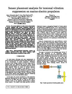
Fig. 2. Sensor placement for a real vehicle detection experiment [8]. The surveillance spots are chosen based on the trajectories of three AAV runs (AAV3-5), which cover the intersection of three roads. The dotted circles are the impact regions of clusters.

surveillance spots in Al . We run the divide-and-conquer algorithm and its refinement process for {Al |1 ≤ i ≤ L} and {Tl |1 ≤ i ≤ L}. When the surveillance spots are densely distributed, L is much smaller than K. Hence, the number of invocations of the CSA solver is reduced from (1+M )·K to (1+M )·L. Moreover, the surveillance spots close to each other are always clustered together and their sensor placement is jointly optimized, which can significantly reduce the total number of sensors.

6

T RACE - DRIVEN S IMULATIONS

We conduct extensive simulations using the real data traces collected in the DARPA SensIT vehicle detection experiments [8]. We refer to [8] for detailed setup of the experiments. The dataset used in our simulations includes the ground truth data and the acoustic signal energy measurements recorded by 17 nodes at a sampling period of 0.75 seconds, when an Assault Amphibian Vehicle (AAV) drives through a road. The ground truth data include the positions of sensors and the track of the AAV recorded by a GPS device. The data traces used in our simulations include the time series recorded for 9 vehicles (AAV3-11). We use the data trace of AAV3 as the training dataset for estimating the energy decay model. The estimated parameters of the signal decay and noise models are: W0 = 0.51 (after normalization), d0 = 2.6 m, k = 2, σ 2 = 0.05. The bounds of false alarm rate and detection probability (i.e., α and β) are set to be 1% and 90%, respectively. The fusion range R is set to be 21 m, which is the optimal value obtained in Appendix D. We choose the surveillance spots based on the trajectories of three AAV runs (AAV3-5), which cover the intersection of three roads as shown in Fig. 2. Specifically, the surveillance spots are chosen regularly on the trajectory of each AAV run with equal distance. The sensor

CDF

1 random (49 sensors) 0.8 random (70 sensors) random (80 sensors) 0.6 D&C (49 sensors) 0.4 0.2 0

60 65 70 75 80 85 90 95 100 Detection probability PD

100 80 60 40 σ2 = 0.05 σ2 = 0.07 σ2 = 0.10

20 0 0.1

0.3

0.5 β

0.7

0.9

180 160 140 120 100 80 60 40 20 0 16

clustered unclustered

The number of sensors N

Fig. 3. The CDF of the Fig. 4. The number of sendetection probabilities at the sors vs. the required detecspots shown in Fig. 2. tion probability. The number of sensors N

placement computed using the clustered-based divideand-conquer approach is plotted in the figure, which has total 49 sensors. Note that the sensor density of our sensor placement is consistent with that of the real deployment in the DARPA SensIT experiments [8]. To evaluate the effectiveness of our placement, we check the coverage of each surveillance spot as follows. For each surveillance spot, the AAV appears for 1000 times and the detection probability is calculated as the ratio of the number of successful detections to the number of appearances of the AAV. As sensors’ positions are different from the real deployment in [8], the real data cannot be directly used in our simulations. When a sensor in the simulation samples an energy measurement, we compute the distance between the sensor and the surveillance spot. The sensor’s measurement is then set to be the real measurement gathered at the same distance to the AAV. We note that such an approach accounts for several realistic factors. For instance, there exists considerable deviation between the measurements of sensors and the analytical signal decay model estimated by the training data. This deviation is due to various reasons including terrain and changing noise levels caused by wind. Moreover, we adopt a baseline sensor placement algorithm. As only the sensors in the fusion region will take part in data fusion, in the baseline algorithm, a certain number of sensors are randomly placed in the union area of the fusion regions of all spots. Fig. 3 plots the Cumulative Distribution Function (CDF) of the detection probabilities at the surveillance spots shown in Fig. 2. The results of our divide-andconquer placement algorithm and the baseline algorithm are labeled with “D&C” and “random”, respectively. We can see from the figure that, with our divide-andconquer placement algorithm, about 90% surveillance spots satisfy the required lower bound of detection probability. There are two reasons for the remaining 10% surveillance spots that do not satisfy the requirement on detection probability. First, the aforementioned deviation between the data traces and the estimated signal decay model can lead to the breach of coverage. Second, although we conduct a large number of detections at each surveillance spot to estimate the detection probability, there still exists deviation between the estimated value and the true detection probability. We can see from Fig. 3 that, when the baseline algorithm places the same number of sensors as ours (i.e., 49 sensors), only 67% surveillance spots satisfy the requirement on detection probability. When the baseline algorithm places up to 80 sensors, its performance is comparable to our solution. Fig. 4 plots the number of sensors placed by our cluster-based divide-and-conquer approach versus the requirement on detection probability, i.e., β. We can see that the number of sensors increases with β. Moreover, if sensors have higher noise level (i.e., greater σ 2 ), more sensors will be required for covering the spots. More extensive evaluation results based on the real data traces can be found in Appendix E.

The number of sensors N

6

25 64 225 The number of spots K (a)

50 45 40 35 30 25 20 15 10 5 20

clustered unclustered

40 100 200 The number of spots K (b)

Fig. 5. The number of sensors vs. the number of spots. (a) Regular spots; (b) Random spots.

7

N UMERICAL R ESULTS

In this section, we conduct numerical experiments to evaluate the performance of the sensor placement algorithms proposed in Section 5. We first evaluate the impact of surveillance spot clustering on our algorithms. We then compare the divide-and-conquer placement algorithm with the global optimal algorithm and a greedy algorithm. More evaluation results on the impacts of fusion radius, impact region radius and decaying factor can be found in Appendix F. The parameters of the signal decay and noise models are set as follows: W0 = 400, d0 = 1, k = 2, σ 2 = 1. The surveillance field A is a 30 × 30 m2 square area. The surveillance spots are chosen regularly (i.e., on regular grid points) or randomly. The bounds of false alarm rate and detection probability (i.e., α and β) are set to be 1% and 90%, respectively. The data fusion range is set to 7.76 m, which is the optimal value derived in Appendix D. The impact region radius is set to be 2R. 7.1 Impact of Clustering We first evaluate the impact of the spot clustering. We run the divide-and-conquer algorithm with and without QT clustering for total 4 regular and 4 random layouts, respectively. The results are shown in Fig. 5(a) and Fig. 5(b). Fig. 5(a) plots the number of placed sensors versus the number of surveillance spots regularly distributed. The curve labeled with “clustered” and “unclustered” represents the results computed by the divideand-conquer placement algorithm with and without QT

4000 3500 3000 2500 2000 1500 1000 500 0

D&C optimal

The number of sensors N

Execution time (seconds)

7

6 8 10 12 14 16 18 The number of sensors N

30

D&C optimal

25 20 15 10 5

6

7 8 9 10 11 12 13 The number of spots K

The number of sensors N

18

The number of sensors N

Fig. 6. Execution time Fig. 7. The number of senvs. the number of sensors sors placed vs. the number placed. of spots. D&C greedy

16 14 12 10 16

25 100 225 The number of spots K

14

D&C greedy

region of the surveillance spot that has the minimum detection probability. The algorithm terminates when every surveillance spot is (α,β)-covered. This algorithm is similar to several greedy sensor placement algorithms employed in previous work [9], [17]. Fig. 8(a) shows the results of 4 random layouts with 4 × 4, 5 × 5, 10 × 10, and 15 × 15 spots. Fig. 8(b) shows the results of four random layouts with 20, 40, 100 and 200 spots. We can see that our cluster-based divide-and-conquer algorithm consistently outperforms the greedy algorithm in all layouts. The average performance gain is about 30%. The visualization of the sensor placements generated by our algorithm and the greedy algorithm can be found in Appendix F.

12

8

10

In this paper, we present both global optimal and efficient divide-and-conquer heuristics for sensor placement problem. By exploiting the unique structure of the problem, the divide-and-conquer algorithms can find nearoptimal solutions at significantly lower cost. We validate our approach through extensive numerical results as well as simulations based on the real data traces collected in a vehicle detection experiment. Our best algorithm runs up to 7-fold faster than the optimal algorithm while using a comparable number of sensors in the placement.

8 6 20

40 100 200 The number of spots K

(a)

(b)

Fig. 8. The number of sensors vs. the number of surveillance spots. (a) Regular spots; (b) Random spots. clustering, respectively. Fig. 5(b) shows the results for random surveillance spots. We can see that the clusterbased placement algorithm can effectively reduce the number of required sensors. For instance, in Fig. 5(a), when there are total 15 × 15 = 225 surveillance spots, 172 sensors are needed without clustering while only 13 sensors are needed when clustering is employed. Another interesting observation is that the number of sensors required does not increase considerably with the number of surveillance spots. For instance, in Fig. 5(b), total 7 sensors are enough to cover 100 surveillance spots, and total 11 sensors are enough to cover 200 surveillance spots. 7.2 Sensor Placement Performance We now compare our divide-and-conquer algorithm against the global optimal algorithm for small networks. Fig. 6 shows the execution time of different algorithms versus the number of sensors placed for seven random surveillance spot layouts. We can see that the divideand-conquer algorithm (labeled as D&C in Fig. 6) is up to 7-fold faster than the global optimal algorithm. Meanwhile, Fig. 7 shows that the divide-and-conquer algorithm places a comparable number of sensors as the optimal algorithm. We also compare our divide-and-conquer algorithm against a greedy algorithm in large-scale networks. In the greedy algorithm, sensors are also organized into detection clusters centered at surveillance spots. In each iteration, we place a sensor randomly in the fusion

C ONCLUSION

ACKNOWLEDGMENTS The work described in this paper was partially supported by the Department of Energy, USA, under grant DOE ER-25737; National Science Foundation, USA, under grants NSF CNS-0954039 (CAREER), NSF IIS0713109, NSF CNS-1017701 (NeTS), and NSF CNS1035773 (CPS); National Basic Research Program of China (973 Program) (No. 2007CB310704); National Natural Science Foundation of China (No. 60821001); Specialized Research Fund for the Doctoral Program of Higher Education (No. 20100005110002); National Science Foundation of China Innovative Grant (70921061); CAS/SAFEA International Partnership Program for Creative Research Teams. We thank Ke Shen for contributing to the early simulations of this work.

R EFERENCES [1] [2] [3]

[4] [5]

D. Li, K. Wong, Y. H. Hu, and A. Sayeed, “Detection, classification and tracking of targets in distributed sensor networks,” IEEE Signal Process. Mag., vol. 19, no. 2, 2002. F. Zhao, J. Shin, and J. Reich, “Information-driven dynamic sensor collaboration for tracking applications,” IEEE Signal Process. Mag., vol. 19, no. 2, 2002. T. He, S. Krishnamurthy, J. A. Stankovic, T. Abdelzaher, L. Luo, R. Stoleru, T. Yan, L. Gu, J. Hui, and B. Krogh, “Energy-efficient surveillance system using wireless sensor networks,” in ACM MobiSys, 2004. K. Chakrabarty, S. Iyengar, H. Qi, and E. Cho, “Grid Coverage for Surveillance and Target Location in Distributed Sensor Networks,” IEEE Trans. Comput., vol. 51, no. 12, 2002. G. Xing, X. Wang, Y. Zhang, C. Lu, R. Pless, and C. Gill, “Integrated coverage and connectivity configuration for energy conservation in sensor networks,” ACM Trans. Sens. Netw., vol. 1, no. 1, 2005.

8

[6] [7] [8] [9] [10] [11]

[12] [13] [14] [15] [16] [17]

T. Yan, T. He, and J. A. Stankovic, “Differentiated surveillance for sensor networks,” in ACM SenSys, 2003. P. Varshney, Distributed Detection and Data Fusion. Spinger-Verlag, 1996. M. F. Duarte and Y. H. Hu, “Vehicle classification in distributed sensor networks,” J. Parallel and Distributed Computing, vol. 64, no. 7, 2004. T. Clouqueur, V. Phipatanasuphorn, P. Ramanathan, and K. K. Saluja, “Sensor deployment strategy for target detection,” in ACM WSNA, 2002. A. Krause, C. Guestrin, A. Gupta, and J. Kleinberg, “Near-optimal sensor placements: maximizing information while minimizing communication cost,” in IEEE/ACM IPSN, 2006. M. Osborne, S. Roberts, A. Rogers, S. Ramchurn, and N. Jennings, “Towards Real-Time Information Processing of Sensor Network Data Using Computationally Efficient Multi-output Gaussian Processes,” in IEEE/ACM IPSN, 2008. H. Choi, J. How, and P. Barton, “An Outer-Approximation Algorithm for Generalized Maximum Entropy Sampling,” in American Control Conference (ACC), 2008. M. Duarte and Y. H. Hu, “Distance based decision fusion in a distributed wireless sensor network,” in ACM IPSN, 2003. D. Li and Y. H. Hu, “Energy based collaborative source localization using acoustic micro-sensor array,” EURASIP J. Applied Signal Processing, no. 4, 2003. B. W. Wah, Y. Chen, and T. Wang, “Simulated annealing with asymptotic convergence for nonlinear discrete constrained global optimization,” J. Global Optimization, vol. 39, 2007. L. Heyer, S. Kruglyak, and S. Yooseph, “Exploring expression data: Identification and analysis of coexpressed genes,” Genome Research, vol. 9, no. 11, 1999. S. S. Dhillon and K. Chakrabarty, “Sensor placement for effective coverage and surveillance in distributed sensor networks,” in IEEE WCNC, 2003. Xiangmao Chang received the B.S. and M.S. degrees in mathematics from Liao Cheng University, China, in 2004, and Beijing Jiaotong University, China, in 2007, respectively. He is currently working toward the Ph.D. degree in the Department of Computer Science at the Beijing University of Posts and Telecommunications, China. His research interests include power management in wireless sensor networks and secure network coding.

Rui Tan received the B.S. and M.S. degrees in automation from Shanghai Jiao Tong University, China, in 2004 and 2007, respectively. He received the Ph.D. degree in computer science from City University of Hong Kong in 2010. He is currently a postdoctoral research associate at Michigan State University. His research interests include collaborative sensing in wireless sensor networks and cyber-physical systems. He is a member of the IEEE.

Guoliang Xing received the B.S. degree in electrical engineering and the M.S. degree in computer science from Xi’an Jiao Tong University, China, in 1998 and 2001, respectively, and the M.S. and D.Sc. degrees in computer science and engineering from Washington University in St. Louis, in 2003 and 2006, respectively. He is an assistant professor in the Department of Computer Science and Engineering at Michigan State University. From 2006 to 2008, he was an assistant professor of computer science at City University of Hong Kong. He is an NSF CAREER Award recipient in 2010. He received the Best Paper Award at the 18th IEEE International Conference on Network Protocols (ICNP) in 2010. His research interests include wireless sensor networks, mobile systems, and cyber-physical systems.

Zhaohui Yuan received the B.S. degree in computer science in 2004 from Huazhong Normal University, and the Ph.D. degree in computer science in 2009 from Wuhan University, both in China. Currently he is an assistant professor in Huadong Jiao Tong University, China. His research interests include wireless sensor networks, real-time and embedded systems and mobile computing.

Chenyang Lu is a Professor of Computer Science and Engineering at Washington University. The author and co-author of more than 100 publications, Professor Lu received an NSF CAREER Award in 2005. Professor Lu is associate editor of ACM Transactions on Sensor Networks, Real-Time Systems, and International Journal of Sensor Networks, and served as Guest Editor of the Special Issue on Real-Time Wireless Sensor Networks of Real-Time Systems and the Special Section on Cyber-Physical Systems and Cooperating Objects of IEEE Transactions on Industrial Informatics. He also served on the organizational committees of numerous conferences such as Program and General Chair of IEEE Real-Time and Embedded Technology and Applications Symposium (RTAS) in 2008 and 2009, Track Chair on Sensor Networks of IEEE Real-Time Systems Symposium (RTSS) in 2007 and 2009, Program Chair of International Conference on Principles of Distributed Systems (OPODIS) in 2010, and Vice Chair on Sensor Networks and Ubiquitous Computing of International Conference on Distributed Computing (ICDCS) in 2011. He is a member of the Executive Committee of IEEE Technical Committee on Real-Time Systems. He received the Ph.D. degree from University of Virginia in 2001, the M.S. degree from Chinese Academy of Sciences in 1997, and the B.S. degree from University of Science and Technology of China in 1995, all in computer science. His research interests include realtime embedded systems, wireless sensor networks, and cyber-physical systems. Yixin Chen is an Associate Professor of Computer Science at the Washington University in St Louis. He received the Ph.D. in Computing Science from University of Illinois at Urbana-Champaign in 2005. His research interests include nonlinear optimization, constrained search, planning and scheduling, data mining, and data warehousing. His work on planning has won First Prizes in the International Planning Competitions (2004 & 2006). He has won the Best Paper Award in AAAI (2010) and ICTAI (2005), and Best Paper nomination at KDD (2009). He has received an Early Career Principal Investigator Award from the Department of Energy (2006) and a Microsoft Research New Faculty Fellowship (2007). Dr. Chen serves on the Editorial Board of IEEE Transactions of Knowledge and Data Engineering and Journal of Artificial Intelligence Research. Yixian Yang received his Ph.D. degree in signal and information processing from Beijing University of Posts and Telecommunications, Beijing, China in 1988. He is currently a Changjiang Scholar and Distinguished Professor with Beijing University of Posts and Telecommunications, Beijing, China. He is also the director of National Engineering Laboratory for Disaster Backup and Recovery, Key Laboratory of Network and Information Attack & Defense technology of MOE, and Information Security Center, State Key Laboratory of Networking and Switching Technology, Beijing University of Posts and Telecommunications. His research interests include network and information security theory and applications, network-based computer application technology, coding theory and technology.