Wireless Sensor Network, 2010, 2, 48-52 doi:10.4236/wsn.2010.21007 Published Online January 2010 (http://www.SciRP.org/journal/wsn/).
Signal Classification Method Based on Support Vector Machine and High-Order Cumulants Xin ZHOU, Ying WU, Bin YANG Zhengzhou Information Science and Technology Institute, Zhengzhou, China Email:
[email protected] Received September 15, 2009; revised November 13, 2009; accepted November 18, 2009
Abstract In this paper, a classification method based on Support Vector Machine (SVM) is given in the digital modulation signal classification. The second, fourth and sixth order cumulants of the received signals are used as classification vectors firstly, then the kernel thought is used to map the feature vector to the high dimensional feature space and the optimum separating hyperplane is constructed in space to realize signal recognition. In order to build an effective and robust SVM classifier, the radial basis kernel function is selected, one against one or one against rest of multi-class classifier is designed, and method of parameter selection using crossvalidation grid is adopted. Through the experiments it can be concluded that the classifier based on SVM has high performance and is more robust. Keywords: High-Order Cumulants, Support Vector Machine, Kernel Function, Signal Classification
1. Introduction Automatic modulation classification (MC) is an intermediate step between signal detection and demodulation, and plays a key role in various civilian and military applications. It is also one of many key technologies in software radio and cognitive radio. The recognition methods in early years are mainly about signal waveform, frequency, transient amplitude and transient phase [1]. The performances of these methods descend quickly when they face to low SNR. Statistical decision and pattern recognition based on statistics are two main methods in approaching MC problem in recent years [2]. The first method is based on hypothesis testing; problem it has to face is that needs to give proper hypothesis and strict data analysis to get the correct decision threshold. The Reference [3] uses neural net to solve MC problem and gets better effect. But because the sample length is limit, the neural net is easy to bring the phenomenon of overlearning and local minimal value. There are some researchers use support vector machine (SVM) to solve MC problem, and get higher classification accuracy [4,5]. But in the two references they neither gave how to select the optimal parameter of SVM classifier and how to construct multi-class SVM. In this paper, we introduce the support vector machine firstly, then research the selection methods of kernel function and its Copyright © 2010 SciRes.
parameter, and study on the multi-classes classification methods, and then apply them to digital signal classification. We also compare the SVM with other common classifiers. The paper is organized as follows: In Section 2, the robust feature extraction based on high-order cumulants is proposed. In Section 3, the multi-classifier based on SVM is designed. The principle of SVM is introduced firstly, then the kernel and parameter selection are given, the method of decomposing multi-class classifier is used. In Section 4, we input the signal feature to multi-class SVM classifier to do experiment. In Section 5, the paper is concluded.
2. Feature Extraction Based on High-Order Cumulants High-order cumulant is a tool of mathematics which describes the high order statistical characteristic of random process. It not only can remove the influence of Gauss noise, but also is robust to the rotation and excursion of the constellation diagram. We suppose the classifier works in the interrelated and synchronization environment. The received signal has carried out carrier frequency synchronization and timing synchronization, but the unknown referenced phased offset exists. The output signal of receiver can be WSN
X. ZHOU Table 1. The cumulants of signals. signal
C40
C42
C63
C40
C63
C42
C42
3
1.36 E 2
1.36 E 2
9.16 E 3
1
33.36
2E 2
2E 2
13E 3
1
21.125
E2
E2
4E 3
1
16
2/4/8FSK
0
0
16
1
13.76
16QAM
4E 3
E2
0.68 E
2
0.68 E
2
2.08 E
3
xi R n , yi 1, 1 , i 1, 2, , n . -1 and +1 denote
two kinds; the optimal classification hyperplane can be expressed as:
Table 2. The cumulants of FSK signals. C21
C42
2FSK
E 2
E 2 4
4FSK
5 E
9 E
8FSK
21E 2
2
2
x F : (w x) b 0
C21
signal
105 E 2 4
where w is support vector, b is translation vector. In order to make classification hyperplane and w one-toone correspondence, we standardize it and let the distance of the sample which is nearest to hyperplane is 1 w . So hyperplane after standardization satisfies:
1 2.78 4.2
min ( w xi ) b 1
expressed as: r (i ) s (i ) n(i ) L
Eak e jc p (i k ) n(i )
(1)
where ak is the sending symbol sequences, L is the observational symbol number, E is the signal average power, c is referenced phase, p (i ) is channel remnant answer, n(i ) is assumed to be complex white Gaussian noise with power 2 . Suppose the emanant signal serial is independent and identically distributed, the different average power has been normalized to 1, the ideal high-order cumulants of these signals can be expressed by Table 1 [6]. Because we calculate the high-order cumulants can not identify 2FSK, 4FSK and 8FSK signal directly, the ratio 2
and C42
Solving the optimal classification hyperplane can be transformed into quadratic optimization problem:
the signal after difference through median filter which is used to classify FSK signals, where is frequency offset.
3. The Classifier Based on Support Vector Machine 3.1. Support Vector Machine (SVM) SVM is basically a two-class classifier based on the idea of “large margin” and “mapping data into a higher dimensional space” [7]. The principle of SVM is to make minimize the structure risk, in the high dimensional feature space, find an optimal discriminant hyperplane with low VC dimension to make the distance between the two
1 (w w ) 2 y i ( w x i b) 1 0
min (w ) s.t.
(4)
The optimal hyperplane is discussed on the condition that samples can be classified linearly, if can not, we will use slack variables i 0 and penalty factor C to resolve generalized optimal classification hyperplane (to classify samples farthest and make the largest classify margin at the same time): n
min (w )
get from each signal in Table 2 is
Copyright © 2010 SciRes.
(3)
i 1,2,, n
k 1
of C21
(2)
2
C42
4
49
classes’ data have large margin. When the feature space is not linear dividable, SVM maps the data into high dimensional feature space with non-linear mapping, and finds the optimal classification hyperplane in high dimensional feature space. Based on the principle of configuration risk minimization, suppose in inner product space F exists two kinds discriminable samples x1 , y1 , x 2 , y2 , , x n , yn ,
2
4ASK 2PSK/ 2ASK 4PSK
ET AL.
1 (w w ) C i 2 i 1
(5)
yi ( w x i b) 1 i 0 0 i
s.t.
where i 1,2,, n , C is a certain constant, it is the control of the punishment of samples which are classified mistakenly. It is a compromise between the proportion of false classified samples and algorithm complexity. According to the equation above and Lagrange theorem, use Kuhn-Tucker condition, the (5) can be transformed into duality problem: max Q( )
n 1 n n i j yi y j xi x j i 2 j 1 i 1 i 1
n i yi 0 , i 1, 2, , n s.t. i 1 0 i C
(6)
WSN
X. ZHOU
50
Use kernel function k (xi , x j ) (xi ) (x j ) , the quadratic problem can be represented by [8]: max Q( )
(7)
The classification threshold b can be gotten by any support vector use (8): n i yi x i w , i 1,2, , n i 1 y ( w x b) 1 0 i i
f ( x ) sgnw x b sgn i yi k ( x i , x ) b (9) xi SV
y ( x ) . i i
i
x i SV
According to optimal problem (7), the complexity of SVM has nothing to do with dimension of feature, but is restricted by the number of samples. SVM needs to compute the kernel functions between every two training samples, to generate a kernel function matrix which has n* n elements, and n is the number of training samples.
3.2. The Selection of Kernel Function In fact, changing kernel parameter is to change mapping function implicitly, and change the complexity of samples’ distribution in feature space. So the selection of kernel function and parameters are very important. There are 3 kinds of kernels that are usually used [8]: 1) Dimensional polynomial kernel of degree d , the expression is: k ( x, y) [( x, y ) p]d
(10)
where p and d are custom parameters; If p 0 and d 1 , it is called linear kernel function. The operation speed of kernel function is fast. 2) Radial basis function kernel, the expression is: x y k ( x , y ) exp 2
2
(11)
where 2 0 , it controls the width of kernel function Copyright © 2010 SciRes.
(12)
where and v are parameters. Only some values satisfy Mercer condition can be used. Because the feature space of radial basis function kernel is limitless, the limit samples in this feature space must be linearly discriminable, so it is most commonly used in classification. In this paper, we also select radial basis function kernel.
3.3. The Parameter Selection of SVM (8)
The optimal classification discriminant function expressed by kernel function is:
where w
and needs to be confirmed. 3) Neural Network kernel function, the expression is: k ( x, y ) tanh ( x, y ) v
n 1 n n i j yi y j k (xi , x j ) i 2 j 1 i 1 i 1
n i yi 0 , i 1, 2, , n s.t. i 1 0 i C
ET AL.
In SVM classifier, the parameter selection of kernel function and penalty factor is very important. The penalty factor C is the optimal compromise with the distance between hyperplane and the nearest training point is farthest and the classification error is least. The parameters of kernel function determine the data mapping into higher dimensional space. There are many parameter selection methods, such as grid searching, GD algorithm, gradient descent algorithm, genetic algorithm, simulated annealing algorithm and so on. The parameter evaluation criterion has k-fold crossvalidation, leave-one-out (LOO), generalized approximate cross-validation (GACV), approximate span bound, margin-radius bound and so on. In this paper, we use k-fold cross-validation to select parameter C , ( 1 2 )of RBF-SVM. Suppose we have n known samples, they construct sample set xi , yi , i 1, 2, , n , yi 1, 1 . In order to
differentiate kernel function, we use l express the k value of the k-fold cross-validation. The steps of k-fold cross-validation are as followed: 1) Divide sample set contains n samples to l subset equally, each subset contains n l samples. 2) Put from the first to (l-1) subset of (l 1)n l samples as training ones, give a smaller value of parameter (C, ), put in (7) and get the solution of Lagrange operator i* ,the samples corresponding to i* which are more than zero are support vectors. 3) Put each i* into: w
2
( l 1) n l
w *T w *
2 i* *j yi y j exp xi x j
i , j 1
b*
1 sv
(l 1) n l y i* yi exp xi x j k ksv i 1
2
where sv is the number of support vector, and the calWSN
X. ZHOU
ET AL.
51
culation of classification threshold b * uses the mean of each SVM. 4) Put the i* , b* and test samples xu , u (l
4. Computer Simulation and Performance Analysis
1) n l 1, , n into classification function (9) to get the
4.1. Experiment Steps
output f (xu ) of each kind, to validate whether f (xu )
steps 2)–5) to get different accuracy of different parame-
The steps of signal classification of SVM based on grid searching parameters selection are as follows: Extract cumulant features of the received sig1) nals, divide the feature vectors equally to training samples and test samples. Select RBF kernel function and a certain 2) multi-classifier design method; initialize 2 and C ; give the parameter search range, use k-fold cross-validation to get the optimal parameter of SVM. Set the optimal parameter according to step 2) 3) of RBF-SVM and train it using training samples. After training, input features of await classifi4) cation signals to classify them.
ter C , . The experience expresses that parameters in-
4.2. Classification Experiment
is in accordance with real output yu . 5) Take from the second to l subset of (l 1)n l samples as training ones, the first subset as test samples, repeat the steps 2)–4). According to the proposed mechanism, until all subsets are tested, it also repeats the above steps l times and calculates the accuracy of crossvalidation. 6) Fix the parameter C , first increase gradually, repeat steps 2)–5); then increase gradually, repeat
crease as exponent is more effect. 7) Get the max validation classification accuracy and corresponding C , , if the accuracy satisfies requirement, then go to step 8); Or search in the range of
C,
continually which is gotten by the maximum validation accuracy and C , gotten by the second maximum validation accuracy. It also repeats step 2)–6) until satisfies the accuracy. 8) Use the satisfied parameter
C,
to train all
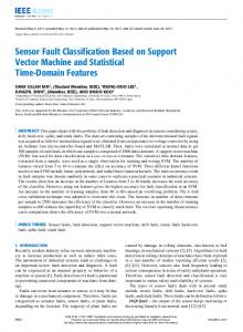
Parameter selection experiment: we create 200 every digital signal every 2dB from 0 to 20dB in awgn channel, extract cumulant feature and get new sample serial. Samples of each class are separated into training ones and test ones randomly. We use SVM one-against-one decomposition, chose RBF kernel, initialize C0 10 ,
02 10 and disperse the parameter logarithmically, get
the grid value log 2 , log C . Where log C {log C0 3, log C0 2, , log C0 3} ,
log 2 log 02 3, log 2 2, , log 2 3 . Then
training samples and get the final optimal parameter
i sv and b , then determine the optimal classification function. * i
*
the isolines of classification accuracy are shown in Figure 1. The maximum accuracy is 99.1% and the optimal parameters are C 0.01 , 2 0.1 .
3.4. The Design of Multi-Classifier
Copyright © 2010 SciRes.
0.98 0. 98
4 0.99
0. 98
0.96
3 0.94 0.9 8
0.9 8
0.99
0. 99
2
0.92
0.9 8
log2
1
0
-1
0.98 0.96 0.94
0.98 0.96 0.94
0.92 0.9
0.88 0.86 0.84 2 0.84 0.8 0.86 0.88 0.9 0.92 0.94 0.96 0.98 0.99
0.88 0.86 0.84
0.98
0.99
0.98 0.96 0.94
0.92 0.9 0.82
0.82 0.84 0.86 0.88 0.9 0.92 0.94 0.96
0.88 0.86 0.84 0.82 0.84 0.86 0.88 0.9 0.92 0.94 0.96
-1
0
1 logC
0.88 0.86 0.84
0.98 8 0.9
-2 -2
0.9
0.92 0.9
0. 9 8
There are two ideas to solve multi-class classification problem of SVM [9]: One is to properly change the original optimal problem in order to compute all the multi-class classification discriminant functions at the same time; the other is to divide the multi-class problem into a series of binary problems which can be solved directly, and based on the results, gain the final discriminant results. The first idea seems to be simpler, but because its computation is too complex and costly, and also hard to implement, it is not widely used. There are 5 kinds of multi-class methods based on the second idea: One Against Rest (OAR), One Against One (OAO), Binary Tree (BT), Error Correcting Output Code (ECOC), Directed Acyclic Graph (DAG). The OAO and OAR methods are often used.
2
3
4
0.82
Figure 1. The cross-validation isolines of OAO-RBF-SVM.
WSN
X. ZHOU
52 Table 3. The simulation result at 5dB. output(classification accuracy) input 4ASK
2PSK/ 2ASK
4PSK
2FSK
4FSK
8FSK
16QA M
4ASK
92.2
7.8
0
0
0
0
0
2PSK/ 2ASK
100
0
0
0
0
0
0
4PSK
0
0.6
99.4
0
0
0
0
2FSK
0
0
0
100
0
0
0
4FSK
0
0
0
2.6
97.4
0
0
8FSK
0
0
0
0.4
2.6
97.0
0
16QAM
0.8
4.2
5.8
0
0
0
89.2
Table 4. Comparison of different classification methods. Classifier
Classification accuracy(%)
Nearest distance classifier
80.2
Neural network
85.6
OAR-SVM
=0.01,C=1
90.4
OAO-SVM
2=0.01,C=0.1
92.2
2
ET AL.
thods of multi-class classifier and method of parameter selection using cross-validation grid search to build effective and robust SVM classifiers. We also use fourth and sixth cumulants of the received signals as the classification vectors, to realize digital signals classification. From the computer simulation and analysis, we can get the following conclusion: 1) The feature vector of cumulants can remove the influence of Gauss noise. It is robust and has high performance. 2) Classification method based on kernel function is less affected by dimension of input data. The classification capability of kernel classifier is affected by the kernel function and parameters, and a fine classification precision can only be obtained when kernel parameters are in special range. The classification stability can be effectively improved by parameter selection via crossvalidate grid search method. If the proper parameters are chosen, the classification accuracy of SVM is high.
6. References [1]
K. Nandi and E. E. Azzouz, “Automatic modulation recognition [J],” Signal Processing, Vol. 46, No. 2, pp. 211– 222, 1995.
Test 1: In this experiment, we get the classification accuracy of different signals in awgn channel. The sample frequency is 40kHz and carrier frequency is 8kHz. The length of signal is 1200, the symbol rate is 2000Bd, and we do 500 Monte Carlo experiments at 5dB. The OAO-SVM is used to get the classification accuracy in Table 3. From Table 3 we can see that SVM classifier can get higher classification accuracy at 5dB. The QAM classification accuracy is lowest and is 89.2%. This is because the feature extraction of QAM is close to the feature of 2PSK and 4PSK, so it is easy to judge to the two signals mistakenly. Test 2: In this experiment, we compare SVM, neural network and the nearest distance discrimination classifier. The simulation assumption is the same as test1. We calculate the classification accuracy of 4ASK at 5 dB. The SVM uses RBF kernel and OAR and OAO classification algorithm, and then we do 500 Monte Carlo experiments. The classification accuracy is shown in Table 4. From Test 2 we can see that the classification accuracy of the nearest distance classifier is lowest, and then is neural network and SVM is highest.
[2]
O. A. Dobre, A. Abdi, Y. Bar-Ness, et al., “Survey of automatic modulation classification techniques: Classical approaches and new trends [J],” IEE Communication, , Vol. 1, No. 2, pp. 137–156, 2007.
[3]
W. C. Han, H. Han, L. N. Wu, et al., “A 1-dimension structure adaptive self-organizing neural network for QAM signal classification [C],” Third International Conference on Natural Computation (ICNC 2007), HaiKou, August 24–27, 2007.
[4]
X. Z. Feng, J. Yang, F. L. Luo, J. Y. Chen, and X. P. Zhong, “Automatic modulation recognition by support vector machines using wavelet kernel [J],” Journal of Physics, International Symposium on Instrumentation Science and Technology, pp. 1264–1267, 2006.
[5]
H. Mustafa and M. Doroslovacki, “Digital modulation recognition using support vector machine classifier [C],” Proceedings of The Thirty-Eighth Asilomar Conference on Signals, Systems & Computers, November 2004.
[6]
O. A. Dobre, Y. B. Ness, and S. Wei, “Higher-order cyclic cumulants for high order modulation classification [C],” IEEE MILCOM, pp. 112–115, 2003.
[7]
Z. L. Wu, X. X. Wang, Z. Z. Gao, and G. H. Ren, “Automatic digital modulation recognition based on support vector machine [C],” IEEE Conference on Neural Networks and Brain, pp. 1025–1028, October 2005.
5. Conclusions
[8]
V. Vapnik, “Statistical learning theory [M],” Wiley, 1998.
[9]
B. Gou and X. W. Huang, “SVM multi-class classification [J],” Journal of Southern Yangtze University, Vol. 21, pp. 334–339, September 2006.
In this paper, we use the kernel thought of statistical learning theory for reference and use decomposition me-
Copyright © 2010 SciRes.
WSN