Simultaneous Localization and Mapping using Multipath ... - CiteSeerX

Simultaneous Localization and Mapping using Multipath Channel Information Erik Leitinger∗,† , Paul Meissner∗,†, Manuel Lafer∗ and Klaus Witrisal∗ ∗

Graz University of Technology, Austria The authors equally contributed to this work.

Simultaneous localization and mapping (SLAM) [1], [2] is all about using uncertain data that are obtained by an agent in some uncertain environment. The uncertainty presents itself on different levels: The measurement data may come from different sensors, giving rise to different measurement variances. When these data are processed by an algorithm, the algorithm needs to take into account this heterogeneity by (i) associating all measurements to their respective origin and (ii) weighting the measurements according to their respective (possibly a-priori unknown) uncertainty. In classical SLAM implementations, much of the measurement origin uncertainty1 is alleviated by using sensors that allow for a resolution of the measurement origin. In the popular example of laser scanners, distance estimates to features are obtained that are labelled with a corresponding angle w.r.t. the pose of the agent. To keep requirements on the agent simple, only single antenna terminals are used in the approach presented here. Hence, only a single signal per anchor (nodes at known positions in the environment) is available per time step. Using an online estimated channel characterization, 1 As

opposed to the inaccuracy of the measurements themselves [3].

Meas. Trajectory Discovered VAs

14

Uncertainty at end

MPC A2, blackboard

Discarded VAs Geom. VAs ≤ order 2

12

Agent tracking

MPC A1, blackboard

10

blackboard 8

(1)

p1

example signal path to VA

6

MPC A1, wind. left windows

4

2

(2)

p1

MPC A1, door and right wind.

right window

I. I NTRODUCTION

16

door

Abstract—Location awareness is one of the most important requirements for many future wireless applications. Multipathassisted indoor navigation and tracking (MINT) is a possible concept to enable robust and accurate localization of an agent in indoor environments. Using a-priori knowledge of a floor plan of the environment and the position of the physical anchors, specular multipath components can be exploited, based on a geometricstochastic channel model. So-called virtual anchors (VAs), which are mirror images of the physical anchors, are used as additional anchors for positioning. The quality of this additional information depends on the accuracy of the corresponding floor plan. In this paper, we propose a new simultaneous localization and mapping (SLAM) approach that allows to learn the floor plan representation and to deal with inaccurate information. A key feature is an online estimated channel characterization that enables an efficient combination of the measurements. Starting with just the known anchor positions, the proposed method includes the VA positions also in the state space and is thus able to adapt the VA positions during tracking of the agent. Furthermore, the method is able to discover new potential VAs in a feature-based manner. This paper presents a proof of concept using measurement data. The excellent agent tracking performance—90 % of the error lower than 5 cm—achieved with a known floor plan can be reproduced with SLAM.

y [m]

†

0 −2

0

2

4

6

8

10

12

14

x [m]

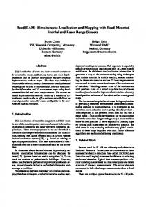
Fig. 1. Illustration of the SLAM approach followed in this paper. Two anchors (1) (2) at p1 and p1 represent the infrastructure. The agent position as well as the floor plan (represented by virtual anchors (VAs)) are estimated using specular multipath, for which one example path is shown. Black squares indicate geometrically expected VAs, blue and red plus markers with uncertainty ellipses (30-fold) represent discovered VAs. An agent tracking result is shown in black with some corresponding ellipses (50-fold). Selected VAs discussed in Section IV are indicated.

measurements from past estimated agent positions are fused efficiently, giving rise to channel information assisted SLAM. The required spatially consistent information about the environment is embedded in the multipath components (MPCs), i.e. the reflections of the signal occurring in the environment [4]. In our prior work [4]–[7], knowledge of the floor plan was assumed to make use of MPCs for localization. In SLAM, however, the floor plan is also subject to the estimation problem. Hence, the aims of this work are (i) to remove the requirement of a precisely a-priori known floor plan and (ii) to cope with uncertainties in the environment representation. The floor plan is represented by virtual anchors (VAs), i.e. mirror images of the positions of the physically existing anchors in the environment [8]. These VAs allow for an efficient representation of the localization-relevant geometry [7]. Fig.

1 illustrates the concept of VAs. For the resulting localization approach, the term multipath-assisted indoor navigation and tracking (MINT) has been coined. Probabilistic MINT flavor is added to the SLAM problem by starting the tracking with just the anchor locations in the environment representation. The MPCs estimated from the received signals of the moving agent over time deliver the spatially consistent geometric data for tracking and for the update of the floor plan2 . All other— not geometrically modelled—propagation effects included in the signals constitute interference to the useful position-related information and are called diffuse multipath (DM) [9]. An online estimation of the influence of the DM on the range uncertainties to the VAs allows for an efficient selection of the VAs that can reliably be updated and used for the agent tracking. This is a key difference to existing radio-based SLAM approaches like [10], [11]. The presented approach can be understood as probabilistic feature-based SLAM [1], [2]. The key contributions of this paper are: • A feature-based method for finding new VAs during tracking of the agent, allowing to infer the floor plan. • Online tracking of VA positions as well as corresponding range uncertainties enables the evaluation of the reliability of the observed features. • A proof-of-concept of the SLAM approach using measured data. The paper is organized as follows: Section II introduces the geometric-stochastic signal model and provides an overview about the subject. Section III describes the components of the SLAM approach, while Sections IV and V wrap up the paper with results, discussions, and conclusions. II. P ROBLEM F ORMULATION A. Signal Model

(j) Kn

=

X

(j)

(j)

(j)

αk,n s(t − τk,n ) + (s ∗ νn(j) )(t) + w(t).

(1)

|αk,n |2

(j)

SINRk,n =

(j)

(j)

N0 + Tp Sν,n (τk,n )

.

(2)

The SINR is used to quantify the position-related information of the k-th MPC. From n this,o the measurement variance of (j) the estimated delay var dˆk,n can be computed (see Section III-C). B. Channel Estimation The MPC arrival time estimation at agent position pn is realized as an iterative least-squares approximation of the received signal [6] Z T 2 (j) (j) (j) τˆk,n = arg min ˆ )s(t − τ ) dt rn (t) − rˆn,k−1 (t) − α(τ τ

A UWB signal s(t) is exchanged between the j-th anchor at (j) position3 p1 ∈ R2 and the agent at position pn ∈ R2 at the n-th time step. The corresponding complex-baseband received signal is modeled as [5] rn(j) (t)

position pn [6]. We assume the energy of s(t) is normalized to one. The second term denotes the convolution of the transmitted (j) signal s(t) with the DM νn (t), which is modeled as a zero-mean Gaussian random process. Note that the statistic (j) of (s ∗ νn )(t) is non-stationary in the delay domain and (j) colored due to the spectrum of s(t). For DM νn (t) we assume uncorrelated scattering along the delay axis τ , hence (j) the nauto-correlation function (ACF) is given by Kν,n (τ, u) = o (j) (j) (j) Eν νn (τ )(νn )∗ (u) = Sν,n (τ )δ(τ − u), where Sν,n (τ ) is the power delay profile (PDP) of DM at the agent position pn . The DM process is assumed to be quasi-stationary in the spatial domain, which means that Sν (τ ) does not change in the vicinity of position pn [12]. Finally, the last term w(t) denotes an additive white Gaussian noise (AWGN) process with double-sided power spectral density (PSD) of N0 /2. Using these channel model parameters, the signal-tointerference-plus-noise ratio (SINR) [5], [6] is defined as

0

(3) using a template signal for all MPCs up to the (k − 1)Pk−1 (j) (j) (j) th defined as rˆn,k−1 (t) = ˆ k′ ,n s(t − τˆk′ ,n ). The k′ =1 α path amplitudes are nuisance parameters, estimated using a (j) projection of rˆn,k (t) onto a unit energy pulse s(t) as Z T (j) (j) (j) α ˆ (τ ) = [ˆ rn,k (t)]∗ s(t − τ )dt; α ˆ k,n = α ˆ (ˆ τk,n ). (4) 0

k=1 (j)

The first term describes a sum of Kn deterministic MPCs (j) (j) with complex amplitudes {αk,n } and delays {τk,n }. We model (j) (j) these delays by VAs at positions pk,n ∈ R2 , yielding τk,n = (j) (j) (j) 1 1 c d(pn , pk,n ) = c kpn − pk,n k with k = 2 . . . Kn , where c (j) (j) is the speed of light. The delay τ1,n = 1c d(pn , p1 ) always defines the direct path between the agent and the j-th anchor. (j) Kn is equivalent to the number of visible VAs at the agent

ˆ n(j) should be chosen The number of estimated MPCs K according to the number of expected specular paths in an environment. With the assumptions of separable MPCs and white noise, (3) and (4) correspond to a maximum-likelihood (ML) estimation of the deterministic MPCs. The finite set of S (j) S (j) Kˆ n(j) measured delays is written as Zn = j Zn = j {dˆk,n }k=1 , (j) (j) ˆ where dk,n = cˆ τk,n . C. General SLAM Formulation

2 We

note that the floor plan itself is not directly estimated, but its representation using the VAs. The reconstruction of the floor plan from this information is out of the scope of this paper. 3 Two-dimensional position coordinates are used throughout the paper, for the sake of simplicity. The extension to three dimensional coordinates is straightforward.

The presented work focuses on probabilistic feature-based SLAM with VAs of the according anchors as representative (j) features of a floor plan. As stated, the VAs at position pk,n (j) are the mirror images of the anchors at position p1 at

flat surfaces, i.e. walls, of the surrounding environment and thus they are a parametric representation of the environment. (j) Starting with the positions of the anchors p1 and optionally a small set of precomputed VAs (using optical ray-tracing [6]), channel information assisted SLAM comprises a method to find new VAs and also to estimate an according reliability (j) measure, the SINRk,n described in Equation (2), for those features. Bayesian feature-based SLAM allows to compute the joint posterior p(xn , An |r1:n ) of the state vector of the agent xn = [pn , vn ]T , where pn is the position and vn the velocity of S (j) the agent, respectively, and An = j An , which represents the finite set of all VA positions at time instance n that are associated with measured delays (see Section III-A). As a consequence of using just one antenna at the anchorand the agent-side, and the partial observability of the VAs, delayed mapping [13] has to be applied, which means that the set of past measurements Z1:n and the according estimated states of the agent x1:n are needed to initialize new possible VAs. In the most generic form, the prediction equation for a feature map and an agent state, using the Markovian assumption, can be written as Z p(xn−1 , An−1 |Z1:n−1 ) p(xn , An |Z1:n−1 ) = xn−1 ,An−1

× p(xn |xn−1 )p(An |An−1 )d{xn−1 , An−1 }

(5)

where p(xn |xn−1 ) and p(An |An−1 ) are the state transition probability distribution functions of the agent and the VAs, respectively. The latter one is represented by an identity function. The update equation is then

well-known multi-target miss-distance, the optimal sub-pattern ˆ n(j) ≥ Kn(j) , which can assignment (OSPA) metric [14]. For K (j) be ensured by filling up Zn with dummy clutter, it is defined as   (j) Kn X 1 (j) (j)   min dOSPA (Dn , Zn ) = ˆ n(j) π∈ΠKˆ (j) K n

where ΠN is defined as the set of permutations of positive integers up to N . The function d(dc ) (x, y) = min(dc , d(x, y)), i.e. an arbitrary distance metric d(·) that is cut off at a dc > 0, the so-called cut-off distance, which is a design parameter. The metric order is denoted as p. The first sum in the metric is the cumulative distance over the optimal sub-pattern assignment (j) (j) (j) (j) of Zn to Dn , i.e. where Kn entries of Zn are assigned (j) optimally to the entries of Dn . The Hungarian or Munkres algorithm can be used for this assignment [14], [15]. For the ˆ n(j) − Kn(j) entries of Zn(j) , dc is assigned as remaining K penalty distance. For performing the data association (DA), we introduce a (j) (j) set Cn of correspondence variables [16], whose i-th entry cn,i is defined as ( (j) (j) k, if dˆi,n corresponds to VA pk (j) (9) cn,i = (j) 0, if dˆ corresponds to clutter. i,n

The optimal sub-pattern assignment between Dn and Zn is reflected by the first part of (8) (j) Kn

π opt = arg min π∈Π ˆ (j) Kn

p(xn , An |Z1:n ) =

p(Zn |xn , An )p(xn , An |Z1:n−1 ) p(Z1:n |Z1:n−1 )

(6)

where p(Zn |xn , A1:n ) represents the general likelihood function of the current measurements. The state space and measurement model that are used in the presented approach are described in Section III-B. III. SLAM A PPROACH The general approach for tracking the agent position and for discovering new VAs is depicted in Fig. 2. This section explains the different parts. A. Data Association (j)

The set of expected MPC delays Dn at time step n is (j) computed as the distances of each VA in An to the predicted position o n (j) (j) . (7) Dn(j) = d(pn,k , pn ) : pn,k ∈ A(j) n (j)

(j)

As Dn and the set of measured delays Zn are sets of usually (j) ˆ n(j) 6= |Dn(j) | = Kn(j) , no different cardinalities, i.e. |Zn | = K conventional distance measure is defined and therefore there is no straightforward way of an association. We employ a

i=1

ip h i p1 (j) p ˆ (j) (j) ) d(dc ) (di,n , dˆ(j) + d ( K − K ) , (8) πi ,n c n n

X

(j)

p d(dc ) (di,n , dˆ(j) π i ,n ) .

(10)

i=1

With this, the correspondence variables are set as ( (j) (j) k, if [π opt ]k = i and d(dc ) (dn,k , dˆn,i ) < dc (j) (11) cn,i = 0, else, where [π opt ]k denotes the k-th entry of the optimal sub-pattern assignment. After the DA was applied for all anchors, the following union sets are defined: • The set of associated discovered (and optionally a-priori S (j) known) VAs An,ass = j An,ass . • The according set of associated measurements Zn,ass = S (j) j Zn,ass . S (j) • The set of remaining measurements Zn,ass = j Zn,ass , which are not associated to VAs of An . B. State Space and Measurement Model The distance estimates for all anchors Zn are stacked in the EKF’s measurement input vector. These measurements are modeled as h iT (j) (j) zn = . . . , d(pn,k , pn ), . . . + nz,n , pk,n ∈ An,ass . (12)

The cardinality of the VA set An,ass is defined as Kn = P (j) j Kn . The vector nz,n contains Gaussian measurement

noise with covariance matrix Rn . The choice of Rn depends on the amount of prior information and will be explained in Section III-C. The tracking of the agent is done as in [17] using an extended Kalman filter (EKF) with DA. We choose a simple linear Gaussian constant-velocity motion model for the agent state xn =Fxn−1 + Gna,n   ∆T 2  1 0 ∆T 0 2  0 1 0 ∆T   xn +  0 =  ∆T 0 0 1 0  0 0 0 1 0

(13) 0



∆T 2  2  na,n .

0  ∆T

The state vector of the agent is xn = [pn , vn ]T , and ∆T is the update rate. The driving acceleration noise term na,n with zero mean and covariance matrix Iσa2 models motion changes that deviate from the constant-velocity assumption. To incorporate the discovered and associated VAs An,ass into the state space, the model is extended to ˜ n na,n ˜ nx ˜ n−1 + G ˜n = F (14) x     F 04×2Kn G ˜ n , = x + 02Kn ×4 I2Kn ×2Kn n−1 02Kn ×2 a,n T T T ˜ n = [xT where x represents the stacked n , p2,n , . . . , pKn ,n ] state vector, where {pk,n } ∈ An,ass . The according measurement model is defined as

˜ nx ˜n + n ˜ z,n , z˜n = H

(15)

T T T where ˜zn = [zT is the stacked n , z2,P2,n , . . . , zKn ,PKn ,n ] measurement vector. The vector zk,Pk,n represents the set of measurements over time that have been associated with the k-th VA, where Pk,n defines the according set of time indices ˜ z,n contains at which the DA was possible. The stack vector n the according measurement noise. The linearized measurement ˜ n is described in Equation (16) on the top of the matrix H next page. Note that (16) shows the general structure of the fully occupied measurement matrix, but for time instance n just columns are present for which the corresponding VAs are in An,ass , and rows for which measurements of zn and zT k,Pk,n ∀ k ∈ An,ass are available. To compute all derivatives ˜ n , also all past agent positions pi i ∈ Pk,n ∀k are needed. in H The covariance matrix Rn contains the according past range variances. The upper left block in (16) comprises the linearized measurement equations for the agent position pn . The other Kn blocks of linearized measurement equations are for the VA (j) positions {pk,n } ∈ An,ass .

C. Range Uncertainty Estimation For the measurement noise modelnof the o tracking filter, the (j) range estimation uncertainties var dˆk,n to the associated VAs are used to build the measurement noise covariance matrix as n n oo (j) (j) Rn = diag var dˆk,n ∀ k, j : pk,n ∈ An,ass . (17)

The MPC range uncertainties can be related to the SINR of the k-th MPC at agent position pn (2) using the Fisher information of the corresponding distances [6] −1  2 2 n o 8π β (j) (j) (j) SINR ≤ var dˆk,n . (18) J−1 (d ) = r k,n k,n 2 c

Here, β denotes the effective (root mean square) bandwidth of s(t). These SINRs are estimated with a method of moments estimator [6] using the associated complex amplitudes (j) {αk,i }ni=n0 over a window of past estimated agent positions where the MPC was associated. The online estimation is started once an initial window size of measurements is available for the respective newly detected 2 VA. Until then, a default value σd,init is assigned. The VA-filter block in Fig. 2 allows to exclude VAs with too unreliable position information, i.e. too large range standard deviation, 2 from the DA, using a threshold value σd,max . For a VA without associated measurements at time step n, the previous value of the estimated range variance is assigned. D. Feature Detection: VA Discovery The set of measurements Zn,ass that are not associated for the tracking phase described above is used for discovering new VAs. In principle, the channel information assisted SLAM algorithm tries to associate these measurements with candidates for new VAs at different stages. This process is illustrated in Figure 2 and is summarized in the following way: ca • The potential subset Zn ⊂ Zn,ass of the non-associated measurements contains measurements that can be associated with already existing VA candidates pca k′ with k ′ = 1, . . . , Cn , which have not yet been estimated unambiguously4. These VA-candidate-associated measureca ca ments {z1,n , . . . , zC } are used to improve the position n ,n estimate of the corresponding VA candidates and to resolve the ambiguity in their positions. • As soon as the position ambiguity is resolved, a new VA is initialized at position pK+1,n 5 , with covariance matrix PK+1,K+1,n and added to the geometry data-base. This new VA can be used in next time step. • Measurements that have not yet been associated with a VA candidate are comprised in Znca and further grouped gr into vectors of similar delays {zgr 1,P1,n , . . . , zGn ,PGn ,n }, where Pg,n represents the set of time-indices of delays associated with the g-th group. Gn is the current number of groups. If the size of a group reaches a certain threshold, a new VA candidate is estimated with the grouped delays and according past agent positions. Estimate new VA candidate pairs: In the case that a vector of similar group delays zgr g,Pg,n has reached a certain number of entries, a new VA candidate pair pca k′ is estimated using the range Bancroft algorithm [18] and the according agent 4 A reason for ambiguity in the position of a newly estimated VA is that the circles spanned by the measured delays around the according agent positions may intersect in two points (e.g. due to agent movement on a straight line). 5 The symbol K defines the number of all discovered VA—until time instance n—that are stored in the geometry memory (see Figure 2).



∂d(p2,n ,pn ) ∂xn

 ..   .  ∂d(pK ,n ,pn ) n   ∂xn   0   .. ˜ Hn =  .   0    0   ..  .  0

∂d(p2,n ,pn ) ∂yn

∂d(p2,n ,pn ) ∂x2,n

∂d(pKn ,n ,pn ) ∂yn

0 0 .. .. . . 0 0

0 .. . 0

0 0 .. .. . . 0 0

0 .. . 0

0 0 .. .. . . 0 0

.. .

Prior knowledge

rn (t)

MPC estim.

∂d(p2,n ,pn ) ∂y2,n

.. . 0

...

0 .. .

0 .. .



.. . 0

...

∂d(p2,n ,p1 ) ∂x2,n

∂d(p2,n ,p1 ) ∂y2,n

∂d(pKn ,n ,pn ) ∂xKn ,n

∂d(pKn ,n ,pn ) ∂yKn ,n

...

∂d(p2,n ,pn−1 ) ∂x2,n

∂d(p2,n ,pn−1 ) ∂y2,n

...

0 .. . 0

0 .. . 0

0 .. . 0

0 .. . 0

...

∂d(pKn ,n ,p1 ) ∂xKn ,n

∂d(pKn ,n ,p1 ) ∂yKn ,n

∂d(pKn ,n ,pn−1 ) ∂xKn ,n

∂d(pKn ,n ,pn−1 ) ∂yKn ,n

.. .

Memory MPCs

.. .

.. .

...

SINR estimation

.. .

           (16)         

2 {σd,k,n }, Z1:n,ass , A− 1:n,ass

Zn

Tracking algorithm

p(xn , An,ass |Z1:n,ass ) b

Zn,ass , An,ass Memory VAs & agent positions

An

VA Filter

A˜n

ˆ− p n

Data Assoc.

Group similar Estimates {zgr g,1:n } New VA Candidate

Memory VAs & agent positions

Zn,ass Znca

Not Assoc. Estimates

ˆ 1:N p

ca Znca → {zc,n }

Pca k′

{pK+1,n , PK+1,K+1,n }

VA Candidate tracking New VA

Fig. 2. Block Diagram of channel information assisted SLAM

1,ca 2,ca positions pPg,n . A VA candidate pair pca k′ = {pk′ , pk′ } is given by the two possible solutions of the range Bancroft method. Tracking of VA candidate pairs: Already found VA candidate pairs Pca k′ are then updated with a recursive least square (RLS) algorithm using the new associated measurements ca ca {z1,n , . . . , zC } and the currently estimated agent position n ,n pn until the above described ambiguities are resolved. Initialize new VA: Resolved VAs are stored in the geometry memory and further used in the state space model. The last update of the RLS algorithm provides the initial position pK+1,n and covariance matrix PK+1,K+1,n of the newly found VA. The cross-covariance PK+1,m,n between the new VA and the agent position and the covariances PK+1,K,n

between the new VA and all other VAs are initialized with zero matrices. IV. R ESULTS For the evaluation of this SLAM approach, we use the seminar room scenario of the MeasureMINT database [19]. We use an agent trajectory as shown in Fig. 1, consisting of 220 points spaced by 5 cm. At each position, UWB measurements of the channel between the agent and the two anchors at the (1) (2) positions p1 and p1 are available. The measurements allow for 25 quasi-parallel trajectories, as in total 25 × 220 points have been measured at a 1 cm grid spacing [6], [7]. These measurements have been performed using an M-sequence correlative channel sounder developed by Ilmsens. This sounder

1 Indiviual runs (SLAM)

0.8

Overall CDF (SLAM) Overall CDF (prior)

CDF

0.6

0.4

0.2

0

0

0.05

0.1 Position error [m]

0.15

0.2

Fig. 3. Performance CDFs for Tp = 0.5 ns and fc = 7 GHz. The grey CDFs indicates the tracking error of the agent using the presented SLAM approach over the 25 trajectories, and the black line denotes the respective overall CDF. Only the anchor coordinates are known. The red dashed line shows the overall CDF using all VAs up to third order as a-priori known and online tracking of their positions and range variances.

provides measurements over the whole FCC frequency range from 3.1 − 10.6 GHz. Out of this range, we select the desired frequency band using filtering with a raised cosine pulse with a pulse duration Tp = 0.5 ns (corresponding to a bandwidth of 2 GHz) at a center frequency of fc = 7 GHz. Fig. 1 shows the final result of the tracking along the trajectory together with the obtained knowledge of the floor plan in terms of the detected VAs and their uncertainties. This is evaluated at the end of the tracking phase for trajectory run 25. Black squares indicate positions of geometrically calculated VAs up to order two. For many of the detected VAs, shown by red (Anchor 1) and blue (Anchor 2) plus markers, there is an underlying expected VA. This is especially the case for these VAs that have a small position variance, indicated by their standard deviation ellipses. The latter are enlarged by a factor of 30 for better visibility. Some detected VAs, e.g. the one at approximately p = [−1.4, 13.4]T , correspond to VAs of order three, which are not shown in the plot. The dark crosses show those detected VAs whose range standard deviation exceeds the threshold of σd,max = 6.23 cm, corresponding to a SINR of 0 dB, c.f. (18) and (2). These are discarded from the tracking process. Some of the detected VAs do not correspond to any geometrically explainable positions, i.e. they represent clutter. This may correspond to scattering objects which are visible for a significant time span. These do not comply to the geometric model of VAs and will be mapped to erroneous positions. However, for many of these false detections, the variance in the position domain is large, in principle allowing for a treatment of these errors on a higher layer. Fig. 3 shows CDFs of the position error of the agent. The grey curves represents the performance of the presented SLAM approach over the 25 individual trajectory runs. Only the two (1) (2) anchor positions p1 and p1 are used as prior knowledge. It can be seen that despite the fact that one run was diverging, the overall performance is excellent, i.e. 90 % of the errors

are within 4.4 cm. As a comparison, the black line shows the overall performance over the 25 runs using all VAs up to order three as prior knowledge. The expected visibility regions of these VAs are precomputed using geometrical raytracing and used in the prediction process to find the set of expected VAs [6], [7]. The corresponding VA positions are tracked using the EKF, and their range variances are estimated online based on the estimated positions of the agent. This provides a performance of 90 % within 3.8 cm, i.e. only slightly better than for SLAM. We suspect that a reason for the good performance of the SLAM approach is that in the VA discovery process, many unreliable MPCs are not detected and thus do not impair the localization. In the case of apriori known VAs, these MPCs will be associated to the signal features and may cause errors. Due to the variance tracking, they should be weighted down after some time, but until then, they influence the tracking. A deeper understanding of the influences as well as an analysis of more measurements to evaluate the significance of the difference is subject of ongoing research. Fig. 4 contains the estimated standard deviations of the ranging to the selected VAs marked in Fig. 1. The default value assigned to newly detected VAs, 0.07 m, is shown (black line) as well as the threshold σd,max that is used to select VAs to become candidates for the data association (grey line). As Fig. 4(a) and (b) show, the blackboard is nicely detectable and usable for tracking, both for Anchor 1 and 2. In the expected regions where the MPC should be invisible, the uncertainty raises, indicating the decrease in position information. For the door and window on the right side and Anchor 1, Fig. 4(c) shows that the corresponding uncertainty is very low. This is expected, as the door is made of metal and the window is metal coated. Interestingly, the estimation continues to yield good values also in the NLOS region. This means that in this region, still a measurement is associated to the discovered VA, otherwise only the previous value is reused. This is an indication of some uncertainty in the geometry, i.e. the reflection from the slightly displaced wall between door and window is associated to the measurement, leading to a VA merging these elements. For the left window and Anchor 2, the estimation is shown in Fig. 4(d). After the VA has been discovered, the variance is estimated well. In the NLOS region, only a few erroneous associations are made, mostly the previous values are used. As the VA becomes visible again, the estimation continues with low uncertainty values. V. C ONCLUSIONS

AND

O UTLOOK

We have presented a proof-of-concept of a SLAM approach that extracts geometry information from single-antenna UWB measurements. We show the general applicability of using information from specular MPCs for localization, without any prior floor plan information. The proposed channel information assisted SLAM algorithm is able to learn efficiently a feature-based representation of the environment using VAs, while tracking the agent position.

0.2

geom. NLOS region σd,k, est.

σd,k [m]

0.15

default val. σd,init thresh. σd,max

0.1

0.05 0

20

40

60

80

100 120 140 time index n

160

180

200

220

ACKNOWLEDGEMENT Part of this work has been funded by the Austrian Research Promotion Agence (FFG) under Grant 845630 “REFlex”.

(a) 0.2

R EFERENCES

σd,k [m]

0.15 0.1

0.05 0

20

40

60

80

100 120 140 time index n

160

180

200

220

160

180

200

220

160

180

200

220

(b) 0.2

σd,k [m]

0.15 0.1

0.05 0

20

40

60

80

100 120 140 time index n

(c) 0.2

σd,k [m]

0.15 0.1

0.05 0

be learned by the SLAM algorithm. In this way, a more structured analysis of influence factors on the performance can be performed. Also, in the initialization of a VA candidate pair, the chosen method may not be optimal. In the case of closely-spaced agent positions, the measurement geometry is often bad, caused by multiple similar circles that do not clearly intersect. A more sophisticated initialization and tracking— using particle filtering and filters based on random finite set statistic—of the candidate positions may help here.

20

40

60

80

100 120 140 time index n

(d) Fig. 4. Estimated standard deviations of the ranging to selected VAs, i.e. the reflections w.r.t. the blackboard and Anchor 1 (a) as well as Anchor 2 (b), the right hand door and window and Anchor 1 (c), and the left window and Anchor 2 (d). Grey regions indicate geometrically computed regions where the corresponding MPC is not visible. Blue lines denote the estimated ranging uncertainty, and black and grey lines the default value and the threshold, respectively.

An important issue for future work is the consideration of synthetic signals in simplified environments. With this, it is easier to provide a ground truth for the geometry that should

[1] H. Durrant-Whyte and T. Bailey, “Simultaneous localization and mapping (SLAM): Part I,” IEEE Robotics and Automation Magazine, vol. 13, no. 2, pp. 99 –110, june 2006. [2] T. Bailey and H. Durrant-Whyte, “Simultaneous localization and mapping (SLAM): Part II,” IEEE Robotics and Automation Magazine, vol. 13, no. 3, pp. 108 –117, sept. 2006. [3] Y. Bar-Shalom and T. Fortmann, Tracking and Data Association. Academic Press, 1988. [4] E. Leitinger, P. Meissner, C. Ruedisser, G. Dumphart, and K. Witrisal, “Evaluation of position-related information in multipath components for indoor positioning,” Selected Areas in Communications, IEEE Journal on, 2014, submitted. [5] K. Witrisal and P. Meissner, “Performance bounds for multipath-assisted indoor navigation and tracking (MINT),” in IEEE International Conference on Communications (ICC), 2012. [6] P. Meissner, E. Leitinger, and K. Witrisal, “UWB for Robust Indoor Tracking: Weighting of Multipath Components for Efficient Estimation,” IEEE Wireless Communications Letters, vol. 3, no. 5, pp. 501–504, Oct. 2014. [7] P. Meissner, “Multipath-Assisted Indoor Positioning,” Ph.D. dissertation, Graz University of Technology, 2014. [8] J. Borish, “Extension of the image model to arbitrary polyhedra,” The Journal of the Acoustical Society of America, 1984. [9] N. Michelusi, U. Mitra, A. Molisch, and M. Zorzi, “UWB Sparse/Diffuse Channels, Part I: Channel Models and Bayesian Estimators,” IEEE Transactions on Signal Processing, 2012. [10] C. Gentner and T. Jost, “Indoor positioning using time difference of arrival between multipath components,” in International Conference on Indoor Positioning and Indoor Navigation (IPIN), Oct 2013, pp. 1–10. [11] T. Deissler and J. Thielecke, “Uwb slam with rao-blackwellized monte carlo data association,” in International Conference on Indoor Positioning and Indoor Navigation (IPIN), Sept 2010, pp. 1–5. [12] A. Molisch, “Ultra-wide-band propagation channels,” Proceedings of the IEEE, 2009. [13] J. J. Leonard, R. J. Rikoski, P. M. Newman, and M. Bosse, “Mapping partially observable features from multiple uncertain vantage points,” The International Journal of Robotics Research, 2002. [14] D. Schuhmacher, B.-T. Vo, and B.-N. Vo, “A Consistent Metric for Performance Evaluation of Multi-Object Filters,” IEEE Transactions on Signal Processing, 2008. [15] J. Munkres, “Algorithms for the Assignment and Transportation Problems,” Journal of the Society for Industrial and Applied Mathematics, vol. 5, no. 1, pp. pp. 32–38, 1957. [16] S. Thrun, W. Burgard, and D. Fox, Probabilistic Robotics. MIT, 2006. [17] P. Meissner, E. Leitinger, M. Froehle, and K. Witrisal, “Accurate and Robust Indoor Localization Systems Using Ultra-wideband Signals,” in European Navigation Conference (ENC), Vienna, Austria, 2013. [Online]. Available: http://arxiv.org/abs/1304.7928 [18] S. Bancroft, “An Algebraic Solution of the GPS Equations,” Aerospace and Electronic Systems, IEEE Transactions on, vol. AES-21, no. 1, pp. 56–59, Jan 1985. [19] P. Meissner, E. Leitinger, M. Lafer, and K. Witrisal, “MeasureMINT UWB database,” 2013, Publicly available database of UWB indoor channel measurements. [Online]. Available: www.spsc.tugraz.at/tools/UWBmeasurements