Keywords Software debugging, Testing, Diagnosis, Logging. Permission to ...... integer program on a MacBook Pro with 2.26 GHz Intel Core 2. Duo and 2GM ...
Software Debugging and Testing using the Abstract Diagnosis Theory Samaneh Navabpour
Borzoo Bonakdarpour
Sebastian Fischmeister
Department of Electrical and Computer Engineering University of Waterloo 200 University Avenue West Waterloo, Ontario, Canada N2L 3G1 {snavabpo, borzoo, sfischme}@ece.uwaterloo.ca
Abstract
1. Introduction
In this paper, we present a notion of observability and controllability in the context of software testing and debugging. Our view of observability is based on the ability of developers, testers, and debuggers to trace back a data dependency chain and observe the value of a variable by starting from a set of variables that are naturally observable (e.g., input/output variables). Likewise, our view of controllability enables one to modify and control the value of a variable through a data dependency chain by starting from a set of variables that can be modified (e.g., input variables). Consequently, the problem that we study in this paper is to identify the minimum number of variables that have to be made observable/controllable in order for a tester or debugger to observe/control the value of another set of variables of interest, given the source code. We show that our problem is an instance of the well-known abstract diagnosis problem, where the objective is to find the minimum number of faulty components in a digital circuit, given the system description and value of input/output variables. We show that our problem is NP-complete even if the length of data dependencies is at most 2. In order to cope with the inevitable exponential complexity, we propose a mapping from the general problem, where the length of data dependency chains is unknown a priori, to integer linear programming. Our method is fully implemented in a tool chain for MISRA-C compliant source codes. Our experiments with several real-world applications show that in average, a significant number of debugging points can be reduced using our methods. This result is our motivation to apply our approach in debugging and instrumentation of embedded software, where changes must be minimal as they can perturb the timing constraints and resource consumption. Another interesting application of our results is in data logging of non-terminating embedded systems, where axillary data storage devices are slow and have limited size.
Software testing and debugging involves observing and controlling the software’s logical behaviour and resource consumption. Logical behaviour is normally defined in terms of the value of variables and the control flow of the program. Resource consumption is defined by both the resources used at each point in the execution and the amount and type of resources used by each code block. Thus, observability and controllability of the state of variables of a software system are the two main requirements to make the software testable and debuggable. Although there are different views towards observability [3, 8– 10, 18–20, 25], in general, observability is the ability to test various features of a software and observe its outcome to check if it conforms to the software’s specification. Different views stand for controllability as well [3, 8–10, 18–20, 25]. Roughly speaking, controllability is the ability to reproduce a certain execution behaviour of the software. The traditional methods for achieving observability and controllability incorporate techniques which tamper with the natural execution of the program. Examples include using break points, interactive debugging, and adding additional output statements. These methods are often unsuited (specially for embedded software), because they cause changes in the timing behaviour and resource consumption of the system. Hence, the observed outcome of the software is produced by a mutated program which can violate its correctness. The mutated program can cause problems for controllability as well. For instance, a previously seen execution behaviour may be hard or impossible to reproduce. Thus, in the context of software testing and debugging, it is highly desirable to achieve software observability and controllability with the least changes in the software’s behaviour. In particular, in embedded software, this property is indeed crucial. This goal becomes even more challenging as the systems grow in complexity, since the set of features to cover during the testing and debugging phase increases as well. This can result in requiring more points of observation and control (i.e., instrumentation) which increases the number of changes made to the program. For instance, testers will require more “printf” statements to extract data regarding a specific feature which causes more side effects in the timing behaviour. With this motivation, we treat the aforementioned problem by first formalizing the notions of observability and controllability as follows. Our view of observability is based on the ability of developers, testers, and debuggers to trace back a sequence of data dependencies and observe the value of a variable by starting from a set of variables that are naturally observable (e.g., input/output variables) or made observable. Controllability is the other side of the
Categories and Subject Descriptors D.2.5 [Software Engineering]: Testing and Debugging —Debugging aids, Dumps, Tracing General Terms Algorithms, Performance, Theory Keywords Software debugging, Testing, Diagnosis, Logging.
Permission to make digital or hard copies of all or part of this work for personal or classroom use is granted without fee provided that copies are not made or distributed for profit or commercial advantage and that copies bear this notice and the full citation on the first page. To copy otherwise, to republish, to post on servers or to redistribute to lists, requires prior specific permission and/or a fee. LCTES’11, April 11–14, 2011, Chicago, Illinois, USA. c 2011 ACM 978-1-4503-0555-6/11/04. . . $10.00 Copyright
coin. Our view of controllability enables one to modify and control the value of a variable through a sequence of data dependencies by starting from a set of variables that can be modified (e.g., input variables). Thus, the problem that we study in this paper is as follows:
reducing the execution time of instrumented code. Indeed, we show that the overall execution time of the code instrumented optimally is significantly better than the corresponding time with the original instrumentation.
Given the source code of a program, our objective is to identify the minimum number of variables that have to be made observable/controllable in order for a tester or debugger to observe/control the value of another set of variables of interest.
Organization. The rest of the paper is organized as follows. After discussing related work in Section 2, in Section 3, we present our notions of observability and controllability and discuss their relevance to software testing and debugging. Section 4 is dedicated to formally present our problem and its complexity analysis. Then, in Section 5, we present a transformation from our problem to ILP. Our implementation method and tool chain are described in Section 6. We analyze the results of our experiments in Section 7. Finally, we make concluding remarks and discuss future work in Section 8.
We show that our problem is an instance of the well-known abstract diagnosis problem [17]. Roughly speaking, in this problem, given are the description of a digital circuit, the value of input/output lines, a set of components, and a predicate describing what components can potentially work abnormally. Now, if the given input/output relation does not conform with the system description, the goal of the problem is to find the minimum number of faulty components that cause the inconsistency. The general diagnosis problem is undecidable, as it is as hard as solving first-order formulae. We formulate our observability/controllability problem as a sub-problem of the diagnosis problem. In our formulation, our objective is not to find which components violate the conformance of input/output relation with the system description, but to find the minimum number of components that can be used to observe/control the execution of software for testing and debugging. Following our instantiation of the abstract diagnosis problem, first, we show that our optimization problem is NP-complete even if we assume that the length of data dependency chains is at most 2. In order to cope with the inevitable exponential complexity, we propose a mapping from the general problem, where the length of data dependency chains in unknown a prior, to integer linear programming (ILP). Although ILP is itself an NP-complete problem, there exist numerous methods and tools that can solve integer programs with thousands of variables and constraints. Our approach is fully implemented in a tool chain comprising the following three phases: 1. Extracting data: We first extract the data dependency chains of the variables of interest for diagnosing from the source code. 2. Transformation to ILP: Then, we transform the extracted data dependencies and the respective optimization problem into an integer linear program. This phase also involves translation to the input language of our ILP solver. 3. Solving the optimization problem: We solve the corresponding ILP problem of finding the minimum set of variables required to diagnose our variables of interest. Using our tool chain, we report the result of experiments with several real-world applications. These applications range over graph theoretic problems, encryption algorithms, arithmetic calculations, and graphical format encoding. Our experiments target two settings: (1) diagnosing all variables involved in a slice of the source code, and (2) diagnosing a hand-selected set of variables typically used by a developer for debugging. Our experiments show that while for the former our method reduces the number of variables to be made directly diagnosable significantly, for the latter the percentage of reduction directly depends upon the structure of the source code and the choice of variables of interest. Since solving complex integer programs is time-consuming, our experimental observations motivate the idea of developing a simple metric in order to intelligently predict whether applying the optimization is likely to be worthwhile. To this end, we propose one such simple metric in this paper and discuss its correlation with our optimization problem. Another beneficial consequence of our optimization is in
2. Related Work As mentioned in the introduction our formulation of the problem is an instance of the abstract diagnosis theory [17]. The diagnosis theory has been extensively studied in many contexts. In [7], Fijany and Vatan propose two methods for solving the diagnosis problem. In particular, they present transformations from a sub-problem of the diagnosis problem to the integer linear programming and satisfiability problems. Our transformation to integer programming in this paper is more general, as we consider data dependency chains of arbitrary length. Moreover, in [7], the authors do not present experimental results and analysis. On the other hand, our method is fully implemented in a tool chain and we present a rigorous analysis of applying the theory on real-world applications. On the same line of research, Abreu and van Gemund [1] propose an approximation algorithm to solve the minimum hitting set problem. This problem is in spirit very close to an instance of the diagnosis problem. The main difference between our work and [1] is that we consider data dependencies of arbitrary length. Thus, our problem is equivalent to a general nested hitting set problem. Moreover, we transform our problem to ILP whereas in [1], the authors directly solve the hitting set problem. Ball and Larus [2] propose algorithms for monitoring code to profile and trace programs: profiling counts the number of times each basic block in a program executes. Instruction tracing records the sequence of basic blocks traversed in a program execution. Their algorithms take the control-flow graph of a given program as input and finds optimal instrumentation points for tracing and profiling. On the contrary, in our work, we directly deal with source code and actual variables. Ball and Larus also mention that vertex profiling (which is closer to our work) is a hard problem and their focus is on edge profiling. Fujiwara [10] defines observability and controllability for hardware. He considers observability as the propagation of the value of all the signal lines to output lines. Respectively, controllability is enforcing a specific value onto a signal line. He notes that if observability and controllability are unsatisfied, additional outputs and inputs must be added to the circuit. This addition is tightly coupled with the position of the line and type of circuit. Moreover, this work does not address how to choose the best point to add pins. In addition, each time the pin counts change, one needs to re-evaluate the observability/controllability of the lines. Freedman [8], Voas, and Miller [25] view observability and controllability from the perspective of black box testing. They consider a function to be observable, if all the internal state information affecting the output are accessible as input or output during debugging and testing. They present the following metric to evaluate obCardinality of input , where DDR should be close servability: DDR = Cardinality of output
to 1 to have observability. Their method affects the temporal behaviour of the software and may expose sensitive information. In the context of distributed systems, the approach in [20, 21] defines a system behaviour to be observable, only if it can be uniquely defined by a set of parameters/conditions. The goal in this work is using deterministic instrumentation with minimal overhead to achieve observability. The shortcoming of this work is that the authors do not present a technique to find the instrumentation with minimal overhead. In addition, the instrumentation should remain in the deployed software to avoid probe effects. Thus, Thane considers a behaviour controllable with respect to a set of variables only when the set is controllable at all times. The author also proposes a real-time kernel to achieve offline controllability. Schutz [18, 19] addresses observability and controllability for time triggered (TT) and event triggered (ET) systems. The author’s method however, does not avoid instrumentation in the design phase and, hence, uses dedicated hardware to prevent probe effects. Schutz argues that TT systems offer alternative flexibility compared to ET systems when handling probe effects caused by enforced observability. Respectively, Schutz shows that unlike ET systems, TT systems have less probe effects in controllability since there is no missing information concerning their behaviour and, hence, an additional approach is needed to collect information. The approach proposed in [6, 15, 16, 23, 24] is in spirit similar to our approach, but in a different setting. The author analyzes the data flow design of a system and define observability and controllability based on the amount of information lost from the input to the output of the system. Their calculations are based on bit-level information theory. This method estimates controllability of a flow based on the bits available at the inputs of the module from the inputs of the software via the flow. Respectively, they estimate observability as the bits available at the outputs of the software from the outputs of the module via the flow. We believe a bit-level information theoretic approach is unsuited for analysis of real-world large applications, because (1) the proposed technique ignores the type of operations constructing the data flow while it has an effect on observing and controlling data, (2) lost bits or corrupted propagated bits throughout a flow may lead us to inconsistent observations, and (3) although the amount of information propagated throughout a flow is of major importance, the bit count is an improper factor of measurement.
3. Observability and Controllability as a Diagnosis Problem The diagnosis problem [17] was first introduced in the context of automatic identification of faulty components of logic circuits in a highly abstract fashion. Intuitively, the diagnosis problem is as follows: Given a system description and a reading of its input/output lines, which may conflict with the description, determine the minimum number of (faulty) components of the system that cause the conflict between the description and the reading of input/output. In other words, the input/output relation does not conform with the system description due to existence of faulty components. Formally, let SD be a system description and IO be the input/output reading of the system, both in terms of a finite set of first-order formulae. Let C be a set of components represented by a set of constants. Finally, let ¬AB (c) denote the fact that component c ∈ C is behaving correctly. A diagnosis for (SD, C, IO) is a minimal set D ⊆ C such that: SD ∧ IO ∧
V
c∈D
AB (c) ∧
V
c∈C−D
¬AB (c)
is satisfiable. Obviously, this satisfiability question is undecidable, as it is as hard as determining satisfiability of a first-order formula.
Our instance of the diagnosis problem in this paper is inspired by Fujiwara’s [10] definition to address observability and controllability1 . Our view is specifically suitable for sequential embedded software where an external entity intends to diagnose the value of a variable directly or indirectly using the value of a set of other variables according to the system description SD. We instantiate the abstract diagnosis problem as follows. We interpret the set C of components as a set of variables. In our context, SD is a set of instructions in some programming language. In order to diagnose the value of a variable v using the value of another variable v ′ , v must depend on v ′ . In other words, there must exist a function F that connects the value of v with the value of v ′ ; i.e., v = F (v ′ ). Thus, we consider the following types of data dependency: 1. Direct Dependency: We say that the value of v directly depends on the value of v ′ iff v = F (v ′ , V ), where F is an arbitrary function and V is the remaining set of F ’s arguments. 2. Indirect Dependency: We say that v indirectly depends on v ′′ iff there exists a variable v ′ , such that (1) v directly depends on v ′ , and (2) v ′ directly depends on v ′′ . Data dependencies can be easily extracted from SD. For example, consider the following program as an instance of SD: (l1) (l2) (l3) (l4) (l5) (l6) (l7) (l8)
g := x + z + y; if g > 100 then c := d / e; else c := f * g; m := x % y; b := d - f; a := b + c;
It is straightforward to see that the value of variable a directly depends on the value of b and c and indirectly on d and g. Observe that the notion of dependency is not necessarily interpreted by left to right assignments in a program. For example, in the above code, the value of variable d directly depends on the value of b and f. On the contrary, one cannot extract the value of x from m and y, as the inverse of the modulo operator is not a function. In our framework, we interpret ¬AB (c) as variable c is immediately diagnosable (i.e., c can be directly observed or controlled). For instance, in programming languages, the value of constants, literals, and input arguments are known a priori and, hence, are immediately diagnosable. Thus, AB (c) means that variable c is not immediately diagnosable, but it may be diagnosed through other variables. To formalize this concept, we define what it means for a variable to be diagnosable based on the notion of data dependencies. Roughly speaking, a variable is diagnosable if its value can be traced back to a set of immediately diagnosable variables. D EFINITION 1 (Diagnosable Variable). Let V be a set of immediately diagnosable variables. We say that a variable v1 , such that AB (v1 ), is diagnosable iff there exists an acyclic sequence σ of data dependencies: σ = hv1 , d1 , v2 i, hv2 , d2 , v3 i, . . . , hvn−1 , dn−1 , vn i, hvn , dn , vn+1 i such that vn+1 ∈ V . In the remainder of this work, we refer to any dependency sequence enabling variable diagnosis as a diagnosis chain. Finally, in our instance of the diagnosis problem, we assume that the predicate IO always holds. As mentioned earlier, our instance of program diagnosis is customized to address variable observability and controllability. Intuitively, a variable is controllable if its value can be defined or 1 Throughout the paper, when we refer to ‘diagnosis’, we mean ‘observabil-
ity/controllability’.
Legend a
a
b
c
d
Variable vertex
Legend
Context vertex l8
Variable vertex
b
Context vertex
c
l7
l2-l5 c1
x
Figure 2. A diagnosis graph.
c2
l3
y
l5 • (Arcs) A = {(u, c) | u ∈ U ∧ c ∈ C ∧ variable v is affected
d
e
f
within context c} ∪ {(c, u) | u ∈ U ∧ c ∈ C ∧ variable v affects context c}.
g l1
x
y
z
Figure 1. A simple diagnosis graph.
modified (i.e., controlled) by an external entity through a diagnosis chain. For instance, if the external entity modifies the value of an immediately diagnosable variable v, then it can potentially modify the value of variables that can be traced back to v. Such an external entity can be the developer, tester, debugger, or the environment in which the program is running. Likewise, a variable is observable if its value can be read through a diagnosis chain. D EFINITION 2 (Controlability). A variable v is controllable iff v is diagnosable and an external entity can modify the value of v by using an immediately controllable variable v ′ and a diagnosis chain that ends with v ′ . D EFINITION 3 (Observability). A variable v is observable iff v is diagnosable and an external entity can read the value of v by using an immediately observable variable v ′ and a diagnosis chain that ends with v ′ . In order to analyze observability and controllability in a more systematic fashion, we introduce the notion of diagnosis graphs. A diagnosis graph is a data structure that encodes data dependencies for a given variable. For instance, with respect to variable a in the above program, all statements but l6 are of interest. In other words, the program slice [4] of the above program with respect to variable a is the set La = {l1, l2, l3, l4, l5, l7, l8}. A special case of constructing slices is for conditional statements (e.g., if-thenelse and case analysis). For example, in the above program, since we cannot anticipate which branch will be executed at runtime, we have to consider both branches to compute dependencies. Thus, for variable c, we take both statements l3 and l5 into account; i.e., Lc = {l2, l3, l4, l5}. Formally, let v be a variable, Lv be a program slice with respect to v, and Vars be the set of all variables involved in Lv . We construct the diagnosis directed graph G as follows. = C ∪ U , where C = {cl | l ∈ Lv } and U = {uv | v ∈ Vars}. We call the set C context vertices (i.e., one vertex for each instruction in Lv ) and the set U variable vertices (one vertex for each variable involved in Lv ).
• (Vertices) V
O BSERVATION 1. Diagnosis graphs are acyclic and bipartite. The diagnosis graph of the above program with respect to variable a is shown in Figure 1. Although our construction of diagnosis graph is with respect to one variable, it is trivial to merge several diagnosis graphs.
4. Statement of Problem and Its Complexity Analysis The notion of diagnosis graph presented in Section 3 can be used to determine several properties of programs in the context of testing and debugging. One such property is whether a debugger has enough information to efficiently observe the value of a set of variables of interest. Another application is in creating data logs. For instance, since it is inefficient to store the value of all variables of a non-terminating program (e.g., in embedded applications), it is desirable to store the value of a subset of variables (ideally minimum) and somehow determine the value of other variables using the logged variables. Such a property is highly valuable in embedded systems as they do not have the luxury of large external mas storage devices. Thus, the problem boils down to the following question: Given a diagnosis graph and a set of immediately diagnosable variables, determine whether a variable is diagnosable. Another side of the coin is to identify a set of variables that can make another set of variables diagnosable. To better understand the problem, consider the diagnosis graph in Figure 1. One can observe the value of a by making, for instance, variables {c, d, f} immediately observable. A valid question in this context is that if a set of variables is to be diagnosed, why not make all of them immediately diagnosable. While this is certainly a solution, it may not be efficient or feasible. Consider again the graph in Figure 1. Let us imagine that we are restricted by the fact that variables {a, b, c, g} cannot be made immediately observable (e.g., for security reasons). Now, in order to diagnose variable a, two candidates are {d, e, f} and {d, f, x, y, z}. Obviously, for the purpose of, for instance, logging, the reasonable choice is the set {d, e, f}. Figure 2 shows another example where choice of variables for diagnosis matters. For instance, in order to make a, b, and c diagnosable, it suffices to make x and y immediately diagnosable. Thus, it is desirable to identify the minimum number of immediately diagnosable variables to make a set of variables of interest diagnosable.
v{a,b}
v{b,c}
v{a,d}
v{b,d}
|V ′ | ≤ K, as K = N in our mapping and |S ′ | ≤ N . Now, since every set s ∈ S is covered by at least one element in S ′ , it implies that V ′ makes all variables in V diagnosable.
v{b}
• (⇐) Let the answer to DGP be the set V ′ ⊆ V . Our claim
Legend
ca
cb
cc
cd
Variable vertex Context vertex
va
vb
vc
vd
Figure 3. An example of mapping HSP to DGP.
It is well-known in the literature that the diagnosis problem is a typical covering problem [1, 7, 17]. In fact, many instances of the diagnosis problem is in spirit close to the hitting set problem [12] (a generalization of the vertex cover problem). We now show that this is indeed the case with respect to our formulation. We also show that a simplified version of our problem is also NP-complete. Instance (DGP). A diagnosis graph G of diameter 2, where C and U are the set of context and variable vertices respectively and A is the set of arcs of G, a set V ⊆ U , and a positive integer K ≤ |U |. Question. Does there exist a set V ′ ⊆ U , such that |V ′ | ≤ K and all variables in V are diagnosable if all variables in V ′ are immediately diagnosable. We now show that the above decision problem is NP-complete using a reduction from the hitting set problem (HSP) [12]. This problem is as follows: Given a collection S of subsets of a finite set S and positive integer N ≤ |S|, is there a subset S ′ ⊆ S with |S ′ | ≤ K such that S ′ contains at least one element from each subset in S? T HEOREM 1. DGP is NP-complete. Proof. Since showing membership to NP is straightforward, we only show that the problem is NP-hard. We map the hitting set problem to our problem as follows. Let S, S, and N be an instance of HSP. We map this instance to an instance of DGP as follows: • (Variable vertices) For each set s ∈ S, we add a variable vertex
vs to U . In addition, for each element x ∈ S, we add a variable vertex vx to U . • (Context vertices) For each element x ∈ S, we add a context
vertex cx to C. • (Arcs) For each element x ∈ S that is in set s ∈ S, we add arc
(vs , cx ). And, for each x ∈ S, we add arc (cx , vx ). • We let V = {vs | s ∈ S} (i.e., the set of variables to be
diagnosed) and K = N . Observe that the diameter of the graph constructed by our mapping is 2. To illustrate our mapping, consider the example, where S = {a, b, c, d} and S = {{a, b}, {b, c}, {a, d}, {b, d}, {b}}. The result of our mapping is shown in Figure 3. We now show that the answer to HSP is affirmative if and only if the answer to DGP is also affirmative: ′
⊆ S. Our claim is that in the instance of DGP, the set V ′ = {vx | x ∈ S ′ } is the answer to DGP (i.e., the set of immediately diagnosable variables). To this end, first, notice that |V ′ | = |S ′ | and, hence,
• (⇒) Let the answer to HSP be the set S
is that in the instance of HSP, the set S ′ = {x | vx ∈ V ′ } is the answer to HSP (i.e., the hitting set). To this end, first, notice that |S ′ | = |V ′ | and, hence, |S ′ | ≤ N , as N = K in our mapping and |V ′ | ≤ K. Now, since every variable vs ∈ V is made diagnosable by at least one variable vertex in V ′ , it implies elements of S ′ hit all sets in S. �
Note that our result in Theorem 1 is for diagnosis graphs of diameter 2. If the diameter of a diagnosis graph is unknown (i.e., the depth of diagnosis chains), we conjecture that another exponential blow-up is involved in solving the problem. In fact, our problem will be similar to a nested version of the hitting set problem and it appears that the problem is not in NP.
5. Mapping to Integer Linear Programming In order to cope with the worst-case exponential complexity of our instance of the diagnosis problem, in this section, we map our problem to Integer Linear Programming (ILP). ILP is a wellstudied optimization problem and there exist numerous efficient techniques for it. The problem is of the form: 8 < Minimize
: Subject to
c.x A.x ≥ b
where A (a rational m × n matrix), c (a rational n-vector), and b (a rational m-vector) are given, and, x is an n-vector of integers to be determined. In other words, we try to find the minimum of a linear function over a feasible set defined by a finite number of linear constraints. It can be shown that a problem with linear equalities or d i s t a n c e 2 ) ? 1 : ( ( d i s t a n c e 1 == d i s t a n c e 2 ) ? 0 : −1);
15 16 17
}
18 19 20 21 22 23 24 25
int main ( i n t a r g c , char ∗ a r g v [ ] ) { s t r u c t m y 3 D V e r t e x S t r u c t a r r a y [MAXARRAY] ; FILE ∗ f p ; i n t i , count =0; int x , y , z ;
26
i f ( a r g c