Solving Decision Problems with Dependent

Journal of Business & Management

Volume 3, Issue 4 (2014), 01-16 ISSN 2291-1995 E-ISSN 2291-2002 Published by Science and Education Centre of North America

Solving Decision Problems with Dependent Criteria by New Fuzzy Multicriteria Method in Excel Jaroslav Ramík1*, Radomír Perzina1 1

Centre of Excellence IT4Innovations, Division of the University of Ostrava, Czech Republic

*Correspondence: Jaroslav Ramík, Centre of Excellence IT4Innovations, Division of the University of Ostrava, IRAFM, 30. dubna 22, 701 03 Ostrava, Czech Republic. E-mail: [email protected] DOI: 10.12735/jbm.v3i4p01

URL: http://dx.doi.org/10.12735/jbm.v3i4p01

Abstract We propose a new MCDM method based on fuzzy pair-wise comparisons and a feedback between the criteria. The evaluation of the weights of criteria, the variants as well as the feedback between the criteria is based on the data given in pair-wise comparison matrices. Extended arithmetic operations with fuzzy numbers are used as well as ordering fuzzy relations to compare fuzzy outcomes. An illustrating numerical example is presented to clarify the methodology. A special SW – Microsoft Excel add-in named FVK was developed for applying the proposed method. Comparing to other software products, FVK is free, able to work with fuzzy data and utilizes capabilities of widespread spreadsheet Microsoft Excel. JEL Classifications: C44, C88 Keywords: multi-criteria decision making, analytic hierarchy process, pair-wise comparisons, feedback, fuzzy numbers

1. Introducation In this paper we propose a new method for solving fuzzy MCDM problems. In some sense the method is parallel to, or, extension of the Analytic hierarchy process (AHP) with feedback between criteria. Instead of the classical eigenvector prioritization method employed in the AHP, here, a fuzzy approach is based on the logarithmic least squares method, i.e. on the geometric-mean aggregation. In (Lootsma, 1993, 1996), it was demonstrated that some notorious occurrences of rank reversal in AHP can be avoided by the geometric-mean aggregation. We also accept the reasons discussed in (Buckley, Feuring, & Hayashi, 2001), and other papers cited therein, for using geometric mean instead of Saaty’s procedures. Our approach is however different to the method by (van Laarhoven & Pedrycz, 1983), and (Lootsma, 1996). The interface between hierarchies, multiple objectives and fuzzy sets have been investigated by the author of AHP T.L. Saaty as early as in (Saaty, 2001). Later on, in (Saaty, 1991, 2001), the author extends the AHP to a more general process with feedback called Analytic Network Process (ANP). In (Mikhailov & Singh, 2003) a new method based on ANP and fuzzy data is proposed, which is, however, essentially different to the approach used in this paper. Recently, (Büyüközkan, Ertay, Kahraman, & Ruyan, 2004), (Enea & Piazza, 2004) and (Mohanty, Agarwal, Choudhury, & Tiwari, 2005), proposed another versions of fuzzy ANP and applied their methods in practice. Here, we propose a relatively simple method based on the original approaches by (Buckley, 1985; Buckley et al., 2001) and (van Laarhoven & Pedrycz, 1983).

~1~

Jaroslav Ramík & Radomír Perzina

Submitted on May 25, 2014

When applying classical MCDM approach on a real decision problem, e.g. when you want to select the best project from the given group of applications, or, to buy the best product for your personal use, say a car or digital camera, one usually meets among others two difficulties:

•

When evaluating pair-wise comparisons (e.g. on the 9-point AHP scale) natural uncertainty is not incorporated;

•

Decision criteria are not independent each other as they should be.

Here, we solve these difficulties by proposing a new method which incorporates uncertainty adopting pair-wise comparisons by triangular fuzzy numbers, and takes into account interdependences between decision criteria, see (Dubois & Prade, 2001). Our method has the following drawbacks and new features comparing to classical AHP/ANP, eventually “fuzzy versions” of AHP, e.g. the one from (van Laarhoven & Pedrycz, 1983), or (Buckley, 1985; Buckley et al., 2001). First, in classical AHP the pairs of elements are evaluated on the scale {1/9, 1/8, ..., 1/2, 1, 2, ...,9}. Here, we extend this scale to the closed interval [1/σ , σ], where σ is arbitrary positive number greater than 1. Moreover, our approach allows for multiple representations of uncertain human preferences: both crisp evaluations, interval, and also fuzzy judgments in the simple form of triangular fuzzy numbers. The proposed method offers a solution from incomplete sets of pair-wise comparisons. By using the geometric average method we derive the resulting weights – relative importance of the elements in the form of triangular fuzzy numbers. When calculating the weights we minimize the measure of uncertainty, i.e. the spreads of fuzzy weights, (Aguarón & Moreno-Jiménez, 2003). This feature, which is new comparing to previous methods, is very important as too large fuzziness of the weights could deteriorate the results. Second, it was already mentioned above, the decision criteria are frequently dependent to each other. For instance, when buying a best product for our personal use, e.g. a car, the price of the car as a decision criterion is interdependent with some other criteria: the power of engine, maintenance cost, quality of design, prestige of the car etc. Evaluating the criteria individually without taking into account dependency between the criteria the result may become misleading. In AHP this problem has been solved by proposing a new methodology – ANP – a general approach for dealing with feedback among decision elements. Here we solve the problem analogically, however, not in the same generality as we do not have suitable tools for handling matrices with fuzzy elements, particularly inverse matrices, eigenvectors etc. We consider only dependences among decision criteria solving the inverse matrix problem by approximating it with the first few terms of Taylor expansion. This approach will help us to overcome the difficulty with interdependent criteria. The paper is structured as follows: Section 2 presents the classical AHP/ANP theory in the suitable vector notation, in Section 3 pair-wise comparison matrices with triangular fuzzy elements are introduced, and in Section 4 we describe an algorithm for calculating fuzzy weights from fuzzy pair-wise comparison matrices. In Section 5 we deal with the problem of inconsistency, we introduce a new inconsistency index for fuzzy pair-wise comparison matrices and finally, in Section 6 we analyze an illustrating example – decision making situation with 3 decision criteria and 3 variants. Also, we supply an illustrating example using a SW tool – Microsoft Excel add-in named FVK developed for applying the proposed method to demonstrate capabilities of the method.

2. Multi-Criteria Decisions and AHP/ANP In classical hierarchical analysis we usually consider a three-level hierarchical decision system: On the first level we consider a decision goal G, on the second level, we have n independent evaluation criteria:

~2~

www.todayscience.org/jbm.php C1, C2,...,Cn, such that

Journal of Business & Management

Vol. 3, Issue 4, 2014

n

∑ w(Ci ) = 1 , where w(Ci) is a positive real number – a weight, usually interpreted i =1

as a relative importance of criterion Ci subject to the goal G. On the third level, m variants (alternatives) of the decision outcomes V1, V2,...,Vm are considered such that again

m

∑ w(V , C ) = 1 , where w(V ,C ) is a r =1

r

i

r

i

non-negative real number – an evaluation (weight) of Vr subject to the criterion Ci, i = 1,2,...,n. It is advantageous to formulate the above mentioned weights into the matrix form, see e.g. (Saaty, 2001).

 w(C1 )     , and W be the m×n Let W1 be the n×1 matrix (weighing vector of the criteria), i.e. W1 = 3    w(Cn )

matrix

 w(C1 ,V1 )  w(Cn ,V1 )  .    W3 =    w(C1 ,Vm )  w(Cn ,Vm ) The columns of this matrix are evaluations of variants according to the criteria. Moreover, W3 is a column-stochastic matrix, i.e. the sums of columns are equal to one. Then Z = W3W1 is an m×1 matrix, i.e. the resulting priority vector of weights of the variants. The variants can be ranked according to these priorities. In real decision systems there exist typical interdependences among criteria or variants. Decision systems with dependences have been extensively investigated by the Analytic Network Process (ANP), see (Saaty, 2001). Consider now the dependences among the criteria. The interdependences of the criteria are characterized by n×n matrix W2

 w(C1 , C1 )  w(Cn , C1 )      W2 =    w(C1 , Cn )  w(Cn , Cn ) .

(1)

Here, the k-th column of W2 is interpreted as the vector of weights characterizing influences of the individual criteria on the k-th criterion and w(Ck,Ck) = 0 as the influence of Ck onto itself is zero. Moreover, n-1 elements of this vector of weights form the vector

w (k)

 w(C k , C1 )        w(C k , C k −1 )  =   w(C k , C k +1 )       w(C k , C n )  , ~3~

(2)

Jaroslav Ramík & Radomír Perzina

Submitted on May 25, 2014

where the elements of w(k) are calculated from the following (n-1)×(n-1) pair-wise comparison matrix

 b1,1    bk −1,1 Bk =  bk +1,1     bn ,1

 

b1, k −1

b1, k +1





 bk −1, k −1 bk −1, k +1  bk +1, k −1 bk +1, k +1  





bn , k −1

bn , k +1

 

b1, n 

   bk −1, n    bk +1, n       bn , n  .

(3)

For all k = 1,2,...,n, bk,k = 1, as Bk is reciprocal (see Section 3).

 W2   is equal to one,  W3 

In (Saaty, 2001), it has been shown that if the sum of every column of matrix  then

Z = W3 (I − W2 ) W1 −1

(4)

is the resulting priority vector of weights of variants applicable for the decision making process, i.e. for ranking the variants. Usually, the matrix W2 is close to the matrix with zero elements and the dependences among criteria are weak, it can be approximated by the first few terms of Taylor’s expansion

(I − W2 )−1 = I + W2 + W22 + ...

(5)

Then by substituting the first four terms from (5) to (4) we get

Z = W3 (I + W2 + W22 + W23 ) W1 ,

(6)

where I is the unit matrix. In the next section, formula (6) will be used for computing fuzzy evaluations of the variants.

3. Fuzzy Numbers and Fuzzy Matrices

~ can be equivalently expressed by a triple of real numbers, i.e. A triangular fuzzy number a a~ = (a L ; a M ; aU ) , where aL is the Lower number, aM is the Middle number, and aU is the Upper number, aL ≤ aM ≤ aU . If ~ is said to be the crisp number (non-fuzzy number). Evidently, the set of all crisp aL = aM = aU, then a numbers is isomorphic to the set of real numbers. In order to distinguish fuzzy and non-fuzzy numbers we shall denote the fuzzy numbers, vectors and matrices by the tilde above the symbol. As ~ is assumed to be piece-wise linear. usual, the membership function of a It is well known that the arithmetic operations +,-, * and / can be extended to fuzzy numbers by the Extension principle, see e.g. (Buckley et al., 2001). In case of triangular fuzzy numbers ~ a~ = (a L ; a M ; a U ) and b = (b L ; b M ; bU ) , aL > 0, bL > 0, we use special formulae ~4~

www.todayscience.org/jbm.php

Journal of Business & Management

Vol. 3, Issue 4, 2014

~ b~ = (a L + b L ; a M + b M ; aU + bU ) – “addition”, a~ + ~

− b = (a L − bU ; a M − b M ; a U − b L ) – “subtraction”, a~ ~ ~~ a~ * b = (a L * b L ; a M * b M ; aU * bU ) – “multiplication”, ~~ a~ / b = (a L / bU ; a M / b M ; a U / b L ) – “division”. It should be noted, that the above formulae for multiplication and also for division are not obtained from the Extension principle. The above stated operations are only approximate ones, it means that the result of e.g. multiplication is a triangular fuzzy number with piece-wise linear membership function, whereas the membership function of the exact operation defined by the Extension principle is non-linear. If all elements of an m×n matrix A are triangular fuzzy numbers we call A the matrix with triangular fuzzy elements and this matrix is composed of triples as follows: U  (a11L ; a11M ; a11 )  (a1Ln ; a1Mn ; a1Un )  ~   A=    . L M U L M U (a m1 ; a m1 ; a m1 )  (a mn ; a mn ; a mn )  

(7)

~

~

Particularly, let A be an n×n matrix with triangular fuzzy elements. We say that A is reciprocal, if

~ = (a L ; a M ; a U ) implies a~ = ( 1 ; 1 ; 1 ) for all i,j = the following condition is satisfied: a ji ij ij ij ij M L U aij aij

aij

1,2,...,n, i.e.: U  (1 ; 1 ; 1) (a12L ; a12M ; a12 )  1 1 1 (1 ; 1 ; 1) ( U ; M ; L ) ~ A =  a12 a12 a12    1 1 1  1 1 1 ( a U ; a M ; a L ) ( a U ; a M ; a L ) 2n 2n 2n  1n 1n 1n

 (a1Ln ; a1Mn ; a1Un )    (a2Ln ; a2Mn ; a2Un ) ,      (1 ; 1 ; 1)  

(8)

L M U where 0 < a ij ≤ a ij ≤ a ij , i,j = 1,2,...,n.

4. Algorithm The proposed method of finding the best variant (or ranking all the variants) can be characterized in the following three steps: 1. Calculate the triangular fuzzy weights from the fuzzy pair-wise comparison matrices. 2. Calculate the aggregating triangular fuzzy evaluations of the variants. 3. Find the “best” variant (eventually, rank the variants). ~5~

Jaroslav Ramík & Radomír Perzina

Submitted on May 25, 2014

Below we explain in details the individual steps. Step 1: Calculate the triangular fuzzy weights from the fuzzy pair-wise comparison matrices. We assume that both the importance of the criteria and values of the criteria and also the feedback between the criteria are given by the fuzzy weights calculated from the corresponding pair-wise comparison matrices with triangular fuzzy elements.

~

Let A be an n×n reciprocal pair-wise comparison matrix with fuzzy elements (8). Following (van Laarhoven & Pedrycz, 1983), we shall calculate a fuzzy vectors of triangular fuzzy weights ~ ~ ,w ~ ,..., w ~ , such that a special distance between A ~ ,w ~ ,..., w ~ is minimized. In and weights w w 1 2 n 1 2 n contrast to (van Laarhoven & Pedrycz, 1983), who used the following functional 2

   wiL wiM L   log − log a + log − log aijM ∑ ij  U M   wj wj i< j   

2

2

U     +  log wi − log aijU  , L    wj   

here, we apply a modification of this well known logarithmic least-squares method for calculating

wkL , wkM , wkU . Particularly, we solve the following optimization problem: 2

   wiL wiM L   − + − log aijM log log log a ∑ ij  L M   w w i< j  j j  

2

2

U     +  log wi − log aijU   → min;    wUj   

(9)

subject to

wkU ≥ wkM ≥ wkL ≥ 0 , k = 1,2,...,n.

(10)

Setting the derivatives of the function in (9) to zero (a necessary condition of optimality), it can be easily shown, that the optimal solution of problem (9), (10) shall satisfy the following relations: 1/ n

 n  w = CL ⋅  ∏ akjL   j =1  L k

1/ n

  n w = CM ⋅  ∏ akjM    j =1 , M k

1/ n

  n wkU = CU ⋅  ∏ akjU   j =1  ,

,

(11)

k = 1, 2,...,n, where coefficients CL, CM, CU are suitable positive constants satisfying the following requirements.

~ = ( wL ; wM ; wU ) satisfy the First, we ask that the middle values wkM of the fuzzy weights w k k k k “normalization condition”, i.e.

n

∑w k =1

M k

= 1 . Hence, from normalization condition and (11) we obtain:

~6~

www.todayscience.org/jbm.php

Journal of Business & Management CM =

1 n

∑ (∏ a i =1

j

Vol. 3, Issue 4, 2014

.

(12)

M 1/ n ij

)

From (10) and (11) we obtain: 1/ n 1/ n  n  n     M M   ∏ aij     ∏ aij        j =1   j =1   . , C L ≤ C M min  max C C ≥  U M 1/ n  1/ n  i =1,..., n i =1,..., n  n U    n L    ∏ aij     ∏ aij   1 j =     j =1   

(13)

~ = ( wL ; wM ; wU ) , k = 1, 2,...,n, with the minimal spread, i.e. Second, we want to find weights w k k k k the minimal measure of fuzziness: sk = wkU − wkL .

(14)

Therefore, by (12) and (13) we choose the resulting weights as follows: 1/ n 1/ n  n    n L M  ∏ akj    ∏ aij         j =1 = j 1    L , where C min = min  wk = Cmin ⋅ 1/ n  1/ n i =1,..., n n n  n      L  ∏ aijM  ∑   ∏ aij     i =1  j =1    j =1  

(15)

1/ n

 n M  ∏ akj    j =1   M , wk = 1/ n n  n   ∏ aijM  ∑   i =1  j =1 

(16)

1/ n 1/ n  n    n U M  ∏ akj    ∏ aij         j =1 j =1    U , where Cmax = max  . wk = Cmax ⋅ 1/ n  1/ n 1 ,..., i n = n n  n      U  ∏ aijM  ∑   ∏ aij     i =1  j =1    j =1  

~

L

M

U

(17)

Particularly, if A is a crisp (i.e. non-fuzzy) matrix, i.e. aij = aij = aij for all i, j, then Cmin = Cmax = 1 , hence wkL = wkM = wkU for all k, and, the solution – weights are crisp, too. ~7~

Jaroslav Ramík & Radomír Perzina

Submitted on May 25, 2014

Remarks 1. 1. The above stated method can be applied both for calculating the triangular fuzzy weights of the criteria and for eliciting relative triangular fuzzy values of the criteria for the individual variants. Moreover, it can be used also for calculating feedback impacts of some criteria on the other criteria. 2. The advantage of our approach is that it usually gives smaller spreads (i.e. fuzziness) of the calculated fuzzy weights. This fact follows from the following inequalities:

0 < xiL ≤ xiM ≤ xiU and

xiL xiL xiM xiU xiU ≤ L ≤ M ≤ U ≤ L for all i, j. xUj xj xj xj xj

3. Eventually, the values of the criteria can be given directly as triangular fuzzy numbers. Then, by the normalization they are transformed again to fuzzy weights. Particularly, assume that evaluations of variants according to some criterion are expressed by triangular fuzzy numbers, ~ , v~ ,..., v~ , moreover, assume that the criterion is maximizing (i.e. “bigger is better”). Let v 1 2 r

v~i = (viL ; viM ; viU ) , i = 1,2,...,r, be a set of triangular fuzzy numbers, e.g. fuzzy evaluations of variants according to some criterion. We assume also 0 < viL ≤ viM ≤ viU . Then we

“normalize” the values to obtain triangular fuzzy weights as follows:

~ = ( wL ; wM ; wU ) , k = 1,2,...,r, w k k k k where L M U ~ =  vk ; vk ; vk  w k S S S   

(18)

r

M and S = ∑ vk . k =1

Step 2: Calculate the aggregating triangular fuzzy evaluations of the variants. Having calculated triangular fuzzy weights from all reciprocal matrices with triangular fuzzy elements as it was described above, we calculate the aggregated triangular fuzzy evaluation of the individual variants. For this purpose we use formula (6) applied to reciprocal matrices with triangular fuzzy elements. We calculate either

~ ~ ~ Z = W3 W1 , if there is no feedback among the criteria, or

~ ~ ~ ~ ~ ~ Z = W3 (I ~ + W2 ~ + W22 ~ + W23 ) W1 , if there is a feedback among the criteria.

~8~

www.todayscience.org/jbm.php

Journal of Business & Management

Vol. 3, Issue 4, 2014

~ (C )  w 1 ~   Here, W1 =    is the vector of fuzzy weights of the individual criteria and the columns of ~ (C )  w n  matrix

~ (C ,V )  ~ (C ,V )  w w 1 1 1 n ~      W3 =   ~ (C ,V )  w ~ (C ,V )  w 1 m n m  ~

are fuzzy evaluations of variants according to the criteria. Similarly, W2 is calculated according to (1) – (3), however, with triangular fuzzy elements. For addition and multiplication of triangular fuzzy numbers we use the fuzzy operations defined earlier. Step 3: Select the “best” variant, or, order the variants. In Step 2 we calculated m variants described as triangular fuzzy numbers, i.e. by the above formula we obtain m triangular fuzzy numbers ( z1L ; z1M ; z1U ),..., ( zmL ; zmM ; zUm ) . Finally, we have to solve the problem of ranking fuzzy variants. As the set of triangular fuzzy numbers is not linearly ordered we have to use some ranking methods. There exist a number of sophisticated methods for ranking fuzzy numbers, for a comprehensive review of ranking methods see e.g. (Chen & Hwang, 1992). Here we present three relatively simple and well applicable ranking methods. The first method for ranking a set of triangular fuzzy numbers is the well known center of gravity method (COG). This method is based on computing the x-th coordinates xig of the center of gravity of every triangle given by the corresponding membership functions of ~ z i , i = 1,2,...,n. Evidently, it holds

ziL + ziM + ziU x = . 3 g i

(19)

By (19) the variants can be ordered from the best (with the highest value of (19)) to the worst (with the lowest value of (19)). The other two ranking methods are based on the α-cut of the triangular fuzzy number, where α∈[0,1] is an aspiration level given by DM. As the α-cut of a triangular fuzzy number ~ z i is an interval [ z iL (α ), z iR (α )] , we can rank the variants either by the left end points of the corresponding intervals, or by their right end points. In the former case we obtain in some sense a pessimistic ranking method (called L-dominant) whereas in the letter case we get an optimistic ranking method of alternatives (R-dominant), see (Ramik, 2007; Ramik & Perzina, 2010). Notice that all three above mentioned ranking methods coincide with the usual ordering of real numbers if the variants are crisp (i.e. non-fuzzy).

5. Illustrating Case Study In this section we analyze an illustrating example – decision making situation with 3 decision criteria ~9~

Jaroslav Ramík & Radomír Perzina

Submitted on May 25, 2014

and 3 variants. Let us assume that the goal of our decision problem is to choose the “best” new shop for our company from 3 pre-selected ones according to 3 criteria: location, suitability for our business, and building design. Location (Criterion 1) concerns surrounding area around the shop. Suitability for our business (Criterion 2) refers to internal structure of the building with respect to our business needs. Building design (Criterion 3) is related to look and feel of the building. The criteria are evaluated by pair-wise comparisons with triangular fuzzy values, moreover, interdependency among them is considered. First, we apply our method, i.e. the algorithm described in Section 4, for solving the decision problem. The evaluation of the weights of criteria, the variants according to criteria as well as the feedback between the criteria is based on the data from fuzzy pair-wise comparison matrices. Here, 1 9

based on the same arguments as in the classical Saaty´s method, we use the scale – interval [ , 9 ] for evaluating preferences between alternatives. We apply, however, triangular fuzzy numbers. Second, for comparison our fuzzy approach with non-fuzzy one, we use also non-fuzzy evaluations in the pair-wise comparisons without feedback. In this case we apply the same approach, i.e. the method based on the geometric-mean aggregation, a particular case of the previous more general situation of crisp evaluations by using the middle numbers aM, i.e. aM = aL = aU. We demonstrate that the results are different comparing to the previous fuzzy approach. Third, we solve the same problem by applying classical AHP by Expert Choice, i.e. we use non-fuzzy evaluations in the pair-wise comparisons without the feedback. Again, we compare the results with the previous cases. A special SW (Microsoft Excel add-in) named FVK was developed for applying the proposed method. Comparing to other software products, FVK is able to work with fuzzy data with capabilities of MS Excel. Here, as a demonstration, we use outputs obtained by this SW. The DM should fill in the grey regions in the corresponding tables; the white regions are calculated automatically. Step 1: Evaluate the pair-wise comparison matrices and calculate the corresponding weights by the geometric-mean aggregation. The data for relative importance of the criteria are given in the following pair-wise comparison matrix:

By (15) – (17) we calculate the corresponding triangular fuzzy weights, i.e. the relative fuzzy importance of the individual criteria:

~ 10 ~

www.todayscience.org/jbm.php

Journal of Business & Management

Vol. 3, Issue 4, 2014

The character of all three criteria is qualitative, they are evaluated by pair-wise comparisons with triangular fuzzy values given in the following 3 pair-wise comparison matrices:

~

The corresponding fuzzy matrix W3 of fuzzy weights – evaluations of variants according to the individual criteria is calculated by (15) – (17) as follows:

The data for evaluations of fuzzy feedbacks between the criteria are given in 3 pair-wise comparison matrices Bk, see formula (3), however, with fuzzy triangular elements. The interpretation of e.g. B1 is as follows: Criterion 1 is “approximately 2 times more influenced” by Criterion 2 than it is influenced by Criterion 3. The term “approximately 2 times more influenced” is evaluated by the triangular fuzzy number (1; 2; 3). ~ 11 ~

Jaroslav Ramík & Radomír Perzina

Submitted on May 25, 2014

By using (15) – (17) we again obtain the corresponding fuzzy weights and arrange these weights ~ into the fuzzy feedback matrix W2 . There are zeros in the main diagonal as we do not expect an impact of the criterion on itself:

Step 2: Calculate the aggregating triangular fuzzy evaluations of the variants. By computing triangular fuzzy weights and evaluations as it was mentioned earlier, we calculate the aggregated triangular fuzzy evaluation of the individual variants. For this purpose we use the approximate formula (6), applied for matrices with the elements being triangular fuzzy numbers – triples of positive numbers and with the normalized columns:

~ ~ ~ ~ ~ ~2~ ~3 ~ Z = W3 (I + W2 + W2 + W2 ) W1 .

(20)

Here, for addition, subtraction and multiplication of triangular fuzzy numbers in (20) we use the fuzzy arithmetic operations defined earlier. Step 3: Select the “best” variant – rank the variants. In Step 2 we have found the variants described as triangular fuzzy numbers, i.e. by (20) we calculated the triangular fuzzy vector

~ = (~ Z z1 , ~z2 , ~z3 ) = (( z1L ; z1M ; z1U ), ( z2L ; z2M ; z2U ), ( z3L ; z3M ; z3U )) given in the following table: ~ 12 ~

www.todayscience.org/jbm.php

Journal of Business & Management

Vol. 3, Issue 4, 2014

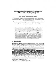
In the following step we have to rank the evaluations of the above fuzzy variants resulting in the “best” variant by using a proper way of ranking the triangular fuzzy numbers depicted in Figure 1. By (19) the variants are ranked from the best (with the biggest value of center of gravity) to the worst (with the lowest value of COG). We can see that by COG method the best variant is Var 2.

Figure 1. Total evaluation of fuzzy variants Now, we solve the same problem applying our method with non-fuzzy evaluations in the pair-wise comparisons and without feedback among the criteria. We apply a particular case of the previous more general situation considering the same data, however, taking into account only middle values of the triangular fuzzy numbers, i.e. aM = aL = aU. Hence, we get

By (19) we obtain the crisp evaluations of the variants:

~ 13 ~

Jaroslav Ramík & Radomír Perzina

Submitted on May 25, 2014

As we can see now the best variant is Var 1. As all three variants are crisp, i.e. real numbers, the above mentioned 3 ranking methods coincide with the natural ordering of real numbers. Now, we solve the same problem with the data as above applying classical AHP by Expert Choice v. 11.0 (with non-fuzzy evaluations in the pair-wise comparisons and without feedback).

We can see that Var 1 is again evaluated as the best one, moreover, numerically the AHP evaluations of the variants are well comparable to the evaluations calculated by our method.

6. Conclusion Considering feedback dependences between the criteria the total rank of the variants may change as we have demonstrated in the above example. Fuzzy (soft) evaluation of pair-wise comparisons may be considered more comfortable and appropriate for DMs. Here, triangular fuzzy numbers have been adopted. A triangular fuzzy number is a natural extension of the crisp number by allowing the left and right spread of uncertainty of the value in question. This flexibility may be advantageous for the DM. An extension to more flexible trapezoidal fuzzy numbers is, of course, possible. By a trapezoidal fuzzy number the DM will define an interval where his/her evaluations are not distinquishable. However, by incorporating trapezoidal fuzzy numbers into our method, the simplicity of the algorithm would be lost. In comparison with other AHP software tools, e.g. Expert Choice, our software FVK is limited to 3 hierarchical levels (goal-criteria-variants) which is most frequent in practice. It cannot be easily extended to more than 3 levels, e.g by adding the level of sub-criteria. In such case, the problem can be reformulated to 3-level problem by combining criteria and sub-criteria. Moreover, the FVK enables to model dependences among criteria which is realistic (and also frequent). A presence of fuzziness in evaluations may change the final rank, when comparing to crisp evaluations of variants in the classical AHP, too. In contrast to the classical AHP which is based on the eigenvector aggregation, our method is based on the geometric-mean aggregation allowing for fuzzy pair-wise comparisons and feedback dependences between the criteria. The evaluation of the weights of criteria, the variants as well as the feedback between the criteria is based on the data given in pair-wise comparison matrices. Extended arithmetic operations with fuzzy numbers are used as well as ordering ~ 14 ~

www.todayscience.org/jbm.php

Journal of Business & Management

Vol. 3, Issue 4, 2014

fuzzy relations to rank fuzzy variants. An illustrating numerical case study is presented to clarify the methodology. A special SW – Microsoft Excel add-in named FVK was developed by the authors of this paper both for solving tentative and real decision makimg problems. Comparing to other software products, FVK is able to work with fuzzy data as well as with capabilities of widespread spreadsheet Microsoft Excel.

Acknowledgements This work was supported by the European Regional Development Fund in the IT4Innovations Centre of Excellence project (CZ.1.05/1.1.00/02.0070).

References [1] Aguarón, J., & Moreno-Jiménez, J. M. (2003). The geometric consistency index: Approximated thresholds. European Journal of Operational Research, 147(1), 137–145. [2] Buckley, J. J. (1985). Fuzzy hierarchical analysis. Fuzzy Sets and Systems, 17(3), 233-247. [3] Buckley, J.J., Feuring, T., & Hayashi, Y. (2001). Fuzzy hierarchical analysis revisited. European Journal of Operational Research, 129(1), 48-64. [4] Büyüközkan, G., Ertay, T., Kahraman, C., & Ruyan, D. (2004). Determining the importance weights for the design requirements in the house of quality using the fuzzy analytic network approach. International Journal of Intelligent Systems, 19(5), 443 – 461. [5] Chen, S. J., & Hwang, C. L. (1992). Fuzzy multiple attribute decision making: Methods and Applications — Lecture notes in economics and mathematical systems (Vol. 375). Berlin, Germany: Springer Berlin Heidelberg. [6] Dubois, D., & Prade, H. (2001). Possibility theory, probability theory and multiple-valued logics: A clarification. Annals of Mathematics and Artificial Intelligence, 32(1-4), 35-66. [7] Enea, M., & Piazza, T. (2004). Project selection by constrained fuzzy AHP. Fuzzy optimization and decision making, 3(1), 39-62. [8] Mikhailov, L., & Singh, M. G. (2003). Fuzzy analytic network process and its application to the development of decision support systems. Systems, Man, and Cybernetics, Part C: Applications and Reviews, IEEE Transactions on, 33(1), 33- 41. [9] Lootsma, F. A. (1993). Scale sensitivity in the Multiplicative AHP and SMART. Journal of Multi-Criteria Decision Analysis, 2(2), 87-110. [10] Lootsma, F. A. (1996). A model for the relative importance of the criteria in the Multiplicative AHP and SMART. European Journal of Operational Research, 94(3), 467-476. [11] Mohanty, R. P., Agarwal, R., Choudhury, A. K., & Tiwari, M. K. (2005). A fuzzy ANP-based approach to R&D project selection: A case study. International Journal of Production Research, ~ 15 ~

Jaroslav Ramík & Radomír Perzina

Submitted on May 25, 2014

43(24), 5199-5216. [12] Ramik, J. (2007). Interval and fuzzy linear programming (demonstrated by example). Paper presented at 25th Internationak Conference Mathematical Methods in Economics, Sep. 04-06, 2007 (pp.290-299). Ostrava, Czech Republic. [13] Ramik, J., & Perzina, R. (2010). A method for solving fuzzy multicriteria decision problems with dependent criteria. Fuzzy Optimization and Decision Making, 9(2), 123-141. [14] Saaty, T. L. (1991). Multicriteria decision making: The analytic hierarchy process — Planning, priority setting, resource allocation. Pittsburgh: RWS Publications. [15] Saaty, T.L. (2001). Decision making with dependence and feedback: The analytic network process — The organization and prioritization of complexity (2nd ed.). Pittsburgh: RWS Publications. [16] van Laarhoven, P. J. M., & Pedrycz, W. (1983). A fuzzy extension of Saaty's priority theory. Fuzzy Sets and Systems, 11(1-3), 199-227.

Copyrights Copyright for this article is retained by the author(s), with first publication rights granted to the journal. This is an open-access article distributed under the terms and conditions of the Creative Commons Attribution 4.0 International License.

~ 16 ~