Solving Non-linear Equations via Genetic Algorithms - CiteSeerX

Proceedings of the 6th WSEAS Int. Conf. on EVOLUTIONARY COMPUTING, Lisbon, Portugal, June 16-18, 2005 (pp24-28)

Solving Non-linear Equations via Genetic Algorithms Nikos E. Mastorakis Head of the Department of Computer Science Military Institutes of University Education (ASEI) Hellenic Naval Academy, Terma Hatzikyriakou 18539, Piraeus GREECE http://www.wseas.org/mastorakis Abstract: - In this paper, a method for solving non-linear equations via GA (Genetic Algorithms) is presented. The method is extended for systems of non – linear equations. The method is compared with a previous one in the literature and it is found that the present one is better. Directions for future research are also provided. Key-Words: - Non – linear equations, genetic algorithms, numerical solutions

1 Introduction Mathematical models for a wide variety of problems in science and engineering can be formulated into equations of the form f ( x) = 0 (1) where x and f ( x) may be real, complex or vector quantities. There exist a great variety of methods to find the roots of (1): a) Analytical methods b) Graphical methods c) Trial and error methods d) Iterative methods. In this paper, we present GA (Genetic Algorithms) methods for solving (1). In section 2, Equation (1) is transformed to a minimization problem and a GA is applied for finding the minimum.

2 Problem Formulation and Solution A brief overview of the GAs methodology could be the following: Suppose that we have to maximize (minimize) the function Q( x) which is not necessary continuous or differentiable. GAs are search algorithms which initially were insiped by the process of natural genetics (reproduction of an original population, performance of crossover and mutation, selection of the best). The main idea for an optimization problem is to start our search no with one initial point, but with a population of initial points. The 2n numbers (points) of this initial set (called population, quite analogously to biological systems) are converted to the binary system. In the sequel, they are considered as chromosomes (actually sequences of 0 and 1).

The next step is to form pairs of these points who will be considered as parents for a "reproduction" (see the following figure)

01100 | 100...11

01100101...10

00011 | 101...10 }→ 00011100...11 parents

children

"Parents" come to "reproduction" where they interchange parts of their "genetic material". (This is achieved by the so-called crossover, see the previous figure) whereas always a very small probability for a Mutation exists. (Mutation is the phenomenon where quite randomly - with a very small probability though - a 0 becomes 1 or a 1 becomes 0). Assume that every pair of "parents" gives k children. By the reproduction the population of the "parents" are enhanced by the "children" and we have an increasement of the original population because new members were added (parents always belong to the considered population). The new population has now 2n+kn members. Then the process of natural selection is applied. According the concept of natural selection, from the 2n+kn members, only 2n survive. These 2n members are selected as the members with the higher values of QQ, if we attempt to achieve maximization of Q (or with the lower values of Q, if we attempt to achieve minimization of QQ). By repeated iterations of

Proceedings of the 6th WSEAS Int. Conf. on EVOLUTIONARY COMPUTING, Lisbon, Portugal, June 16-18, 2005 (pp24-28)

reproduction (under crossover and mutation) and natural selection we can find the minimum (or maximum) of Q as the point to which the best values of our population converge. The termination criterion is fulfilled if the mean value of Q in the 2n-members population is no longer improved (maximized or minimized). More detailed overviews of GAs can be found in [1], [2], [3] and [4] In this paper, our problem is the solution of the equation f ( x) = 0 (1) To this end, the square function Q( x)

Q( x) = f ( x) ≥ 0

If the global minimum of Q( x) is 0 at the point * * * ( x1 , x2 ,L, xn )

*

*

*

then x1 , x2 ,L, xn is a solution

of (4) Another method for solving (4) is min( f1 + f 2 + ... + f n ) under the constraints f1 ( x) ≥ 0, f 2 ( x) ≥ 0,L, f n ( x) ≥ 0 (method developed by Angel Kuri – Morales, [5])

In this paper, we can see that the proposed methodologies are better than the methodology of Angel Kuri – Morales, [5]). Let us consider the following example

2

(2)

is considered. We can find a solution of (1) by finding the global minimum of Q( x) in (2). This minimization is achieved by GA (Genetic Algorithm). A slightly different method can be developed using Q( x) = f ( x) ≥ 0 (3) demanding minimization of Q(x) . Note that the absolute value in (3) does not cause problem in our GA since GA’s do not require the differentiability of the objective function. Another method for solving (1) is the method developed by Angel Kuri – Morales in [5] and is described as follows:

min f ( x)

under the constraint f ( x) ≥ 0 (or

Consider the system of the equations x1 + x1 ⋅ x 2 − 6 = 0 2

(5)

x1 + x 2 + 2 ⋅ x1 ⋅ x 2 − 3 = 0 2

3

2

1st method We demand 2 2 3 2 min( x1 + x1 ⋅ x 2 − 6) 2 + ( x1 + x 2 + 2 ⋅ x1 ⋅ x 2 − 3) 2

2nd method We demand min x1 + x1 ⋅ x 2 − 6 + x1 + x 2 + 2 ⋅ x1 ⋅ x 2 − 3 2

2

3

2

f ( x) ≤ 0 ). The previous ideas can also be extended in the case of a system of n equations in n unknown variables. f1 ( x1 , x2 ,..., xn ) = 0

f 2 ( x1 , x2 ,..., xn ) = 0

(4)

M

f n ( x1 , x2 ,..., xn ) = 0

3rd method (Method Angel – Kuri Morales) We demand 2 2 3 2 min( x1 + x1 ⋅ x 2 − 6 + x1 + x 2 + 2 ⋅ x1 ⋅ x 2 − 3) under the constraints x1 + x1 ⋅ x 2 − 6 ≥ 0 and 2 3 2 x1 + x 2 + 2 ⋅ x1 ⋅ x 2 − 3 ≥ 0 2

The square function Q( x) = f1 + f 2 + L + f n the absolute value function Q( x) = f1 + f 2 + L + f n are defined (or in r general any suitable norm of f = ( f1 , f 2 ,..., f n ) ) and our problem is min Q( x) 2

or

2

2

The following figures show the results in each case. where the following notation is used

Proceedings of the 6th WSEAS Int. Conf. on EVOLUTIONARY COMPUTING, Lisbon, Portugal, June 16-18, 2005 (pp24-28)

Fga = ( x1 + x1 ⋅ x2 − 6) 2 + ( x1 + x2 + 2 ⋅ x1 ⋅ x2 − 3) 2 2

2

3

2

for the first method

Fga = x1 + x1 ⋅ x2 − 6 + x1 + x2 + 2 ⋅ x1 ⋅ x2 − 3 2

2

3

2

for the second method

Fga = x1 + x1 ⋅ x 2 − 6 + x1 + x 2 + 2 ⋅ x1 ⋅ x2 − 3 for the third method 2

2

3

2

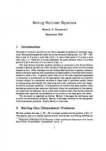
In each case (i.e. in each method) we use: n = 20 (i.e. the number of parents is 2 n = 40) k=4 p mutation = 0.1 (probability for mutation in every generation) Also our chromosome is of 20 bits And we search for x1 , x 2 in the range -100, +100 That means: x1 ∈ [−100,100], x 2 ∈ [−100,100]

Fig.2: 2nd Method

We have the following results (in the horizontal axis we present the number of generations, i.e. iterations of the GA)

Fig.3: 3rd Method

Method

Fga

x1

x2

1st

0.00003591

-2.17316835

-0.59035358

2nd

0.00061440

-2.17206208

-0.59006747

3rd

0.05382000

-3.08009441

1.13125909

Fig.1: 1st Method That means that the first method is better than that of [5]. On the other hand the 3rd method has a serious disadvantage. It cannot converges to x1 = −2.17 and

x2 = −0.59 , because x1 = −2.17 and x2 = −0.59 the following constraint (inequality) fails 2 x1 + x1 ⋅ x 2 − 6 ≥ 0

Proceedings of the 6th WSEAS Int. Conf. on EVOLUTIONARY COMPUTING, Lisbon, Portugal, June 16-18, 2005 (pp24-28)

h1 = ∆x1 , h2 = ∆x 2 ,L, hn = ∆x n

3 Determining all possible roots 3.1 Case of one equation

[

elementary cell

Step1: Choose lower limit a and upper limit b of the interval covering all the roots.

Note that x1 = x1 + N1h1

Step 2: Decide the size of the incremental interval h = ∆x Step 3: Set x1 := α and x2 := x1 + h

hi =

xi − xi i = 1,2,L, n and considering the Ni

C k1 ,k2 ,Lkn = [x1 + k1h1 , x1 + k1h1 + h1 ]×

[x 2 + k 2 h2 , x 2 + k 2 h2 + h2 ]× L × [x n + k n hn , x n + k n hn + hn ]

x2 = x 2 + N 2 h2 xn = x n + N n hn where

Step 4: Compute f1 := f ( x1 ) and f 2 := f ( x2 )

0 ≤ k1 ≤ N1 − 1, 0 ≤ k 2 ≤ N 2 − 1,L, 0 ≤ k n ≤ N n − 1

If f1 , f 2 are of the same sign (i.e

Step 5:

]

Consider that x i , x i has been divided into N i parts, i.e.

The previous developed methodology estimate only one root. If we are interested for all the roots, we can use the so called “incremental search” [6] as follows. Let’s start with one equation like (1). We choose a lower limit a and an upper limit b of the interval covering all the roots. We also have to choose the size of incremental interval ∆x . A major problem is to decide the increment size ∆x . A small ∆x means more iterations, more execution time, but we avoid missing some root or roots. Our algorithm for determining all possible roots of (1) is formulated as follows:

f1 ⋅ f 2 > 0 ) (that means the interval [x1 , x2 ] does

(7)

not bracket any root), then go to Step 7

So S in (6) has been devided into N1 N 2 L N n elementary cells.

Step 6: Apply GA and find the root x * inside the interval [x1 , x2 ] .

We examine the sign of f1 , f 2 ,L f n on the 2 n edge points of each cell. If at least one f i maintains the

If x2 + h < b then set x1 := x2 and

same sign on the 2 n edge points (e1 , e2 ,..., en ) of the elementary cell C k1 ,k2 ,Lkn of (7) then: do not seek

Step 7:

x2 := x2 + h and go to Step 4

for possible roots of (4) in C k1 ,k2 ,Lkn , do not apply

Step 8: Stop

the GA and go to next cell. Note that: (e1 , e2 ,..., en ) are the 2 n edge points

3.2 Case of system of equations Suppose that the system of equations are as in (4). We choose lower limit and upper limit for each variable say: x i , x i for i = 1,2,L, n That means that we seek roots in the closed subset

[

][

]

[

]

S = x1 , x1 × x 2 , x 2 × L × x n , x n ⊂ Iℜ n

e1 = x1 + k1h

or

x1 + k1h + h1

e2 = x 2 + k 2 h

or

x 2 + k 2 h + h2

en = x n + k 2 h

M or

x n + k 2 h + h2

(6)

A generalized incremental search can be achieved considering the incremental intervals

If each f i change signs on the 2 n edge points (e1 , e2 ,..., en ) of the elementary cell C k1 ,k2 ,Lkn of (7) then seek for a root of (4) inside C k1 ,k2 ,Lkn by applying GA.

Proceedings of the 6th WSEAS Int. Conf. on EVOLUTIONARY COMPUTING, Lisbon, Portugal, June 16-18, 2005 (pp24-28)

Repeat this procedure until exhausting all the N1 N 2 L N n elementary cells.

4 Conclusion GA (Genetic Algorithms) is really a powerful tool for many problems in numerical analysis and scientific computation. In this paper, we apply GA to solve a non-linear equation as well as systems of non-linear equations. Work is in progress by the author in the direction of applying Gas in many open problems of numerical analysis such a polynomial factorization, solution of differential equations, etc. See [7]÷[10]. Other relevant studies can be found in [11], [12].

References: [1] Goldberg D.E. (1989), Genetic Algorithms in Search, Optimization and Machine Learning, Addison-Wesley, Second Edition, 1989 [2] Grefenstette J.J., Optimization of control parameters for Genetic Algorithms, IEEE Trans. Systems, Man and Cybernetics, SMC 16, Jan/Feb 1986, pp. 128 [3] Eberhart R., Simpson P. and Dobbins R. (1996), Computational Intelligence PC Tools, AP Professionals. [4] Kosters W.A., Kok J.N. and Floreen P., Fourier Analysis of Genetic Algorithms, Theoretical Computer Science, Elsevier, 229, 199, pp. 143175. [5] Angel Fernando Kuri-Morales, “Solution of Simultaneous Non-Linear Equations using Genetic Algorithms”, WSEAS Transactions on SYSTEMS, Issue 1, Volume 2, January 2003, pp.44-51 [6] E. Balagusuramy, Numerical Methods, Tata McGraw Hill, New Delhi, 1999 [7] Ioannis F. Gonos, Lefteris I. Virirakis, Nikos E. Mastorakis, M.N.S. Swamy, "Evolutionary Design of 2-Dimensional Recursive Filters via the Computer Language GENETICA" to appear in IEEE Transactions on Circuits and Systems I: Fundamental Theory and Applications. (2005) [8] Gonos I.F., Mastorakis N.E., Swamy M.N.S.: “A Genetic Algorithm Approach to the Problem of Factorization of General Multidimensional Polynomials”, IEEE Transactions on Circuits and Systems I: Fundamental Theory and Applications, Part I, Vol. 50, No. 1, pp. 16-22, January 2003.

[9] Mastorakis N.E., Gonos I.F., Swamy M.N.S.: “Design of 2-Dimensional Recursive Filters using Genetic Algorithms”, IEEE Transactions on Circuits and Systems I: Fundamental Theory and Applications, Part I, Vol. 50, No. 5, pp. 634-639, May 2003. Mastorakis N.E., Gonos I.F., Swamy [10] M.N.S.: “Stability of Multidimensional Systems using Genetic Algorithms”, IEEE Transactions on Circuits and Systems, Part I, Vol. 50, No. 7, pp. 962-965, July 2003. [11] I. F. Gonos and I. A. Stathopulos, “Estimation of multi-layer soil parameters using genetic algorithms”, IEEE Transactions on Power Delivery, vol. 20, no. 1, Jan. 2005. [12] I. F. Gonos, F. V. Topalis and I. A. Stathopulos, “A genetic algorithm approach to the modeling of polluted insulators”, IEE Proceedings Generation, Transmission and Distribution, vol. 149, No. 3, May 2002, pp. 373-376.