Source-Level IP Packet Bursts: Causes and Effects∗ Hao Jiang
Constantinos Dovrolis
College of Computing Georgia Institute of Technology
College of Computing Georgia Institute of Technology
[email protected]
[email protected]
ABSTRACT By source-level IP packet burst, we mean several IP packets sent back-to-back from the source of a flow. We first identify several causes of source-level bursts, including TCP’s slow start, idle restart, window advancement after loss recovery, and segmentation of application messages into multiple UDP packets. We then show that the presence of packet bursts in individual flows can have a major impact on aggregate traffic. In particular, such bursts create scaling in a range of timescales which corresponds to the burst duration. Uniform “spreading” of bursts in the time axis reduces the scaling exponent in short timescales (up to 100-200ms) to almost zero, meaning that the aggregate traffic becomes practically uncorrelated in that range. This result provides a plausible explanation for the scaling behavior of Internet traffic in short timescales. We also show that removing packet bursts from individual flows reduces significantly the tail of the aggregate marginal distribution, and it improves queueing performance, especially in moderate utilizations (50-85%). Categories and Subject Descriptors: C.2.3 [Network Operations]: Traffic modeling and analysis General Terms: Measurement, Performance Keywords: scaling, network traffic, TCP, packet dispersion, packet trains, capacity estimation, correlation structure
1.
INTRODUCTION
By source-level IP packet burst, we mean several IP packets sent back-to-back, i.e., at the maximum possible rate, from the source of a flow. Source-level bursts introduce strong correlations in the packet interarrivals of individual flows. Which protocol mechanisms create such bursts? Over ∗This work was supported by the “Scientific Discovery through Advanced Computing” (SciDAC) program of DOE (DE-FC02-01ER25467), and by an equipment donation from Intel Corporation.
Permission to make digital or hard copies of all or part of this work for personal or classroom use is granted without fee provided that copies are not made or distributed for profit or commercial advantage and that copies bear this notice and the full citation on the first page. To copy otherwise, to republish, to post on servers or to redistribute to lists, requires prior specific permission and/or a fee. IMC’03, October 27–29, 2003, Miami Beach, Florida, USA. Copyright 2003 ACM 1-58113-773-7/03/0010 ...$5.00.
which timescales do the corresponding correlations extend? Significant research efforts have focused recently on the correlation structure, or scaling behavior, of aggregate IP traffic in short timescales, typically up to a few hundreds of milliseconds [1, 2, 3, 4]. Is the short time scaling behavior of aggregate traffic related to the presence of packet bursts in individual flows? How will the correlation structure of aggregate traffic change if flows do not include such bursts? In terms of network performance, how will the queueing delays decrease if we remove bursts from individual flows, and in what load conditions is such a decrease most important? These are some of the questions that we investigate in this paper. Background on scaling. The key tool that we rely on is the wavelet-based multiresolution analysis developed in [5] and implemented in [6]. This statistical tool allows us to observe the scaling behavior of a traffic process over a certain range of timescales. Consider a reference timescale T0 , and let Tj =2j T0 for j=1,2,. . . be increasingly coarser timescales. These timescales, or simply scales, partition a traffic trace in consecutive and non-overlapping time intervals. If tji is the i’th time interval at scale j>0, then tji consists of the j intervals tj−1 and tj−1 2i 2i+1 . Let Xi be the amount of traffic in j−1 j−1 j j ti , with Xi = X2i + X2i+1 . The Haar wavelet coefficients {dji } at scale j are defined as j−1 j−1 dji = 2−j/2 (X2i − X2i+1 )
(1)
for i = 1, . . . Nj , where Nj is the number of wavelet coefficients at scale j. The energy function E j is defined as Ej = E[(dji )2 ] ≈
j 2 i (di )
Nj
(2)
An energy plot, such as Figure 1, shows the logarithm of the energy E j as a function of the scale j. The magnitude of E j increases with the variability of the traffic process X j−1 at scale j-1. What is more important is the scaling behavior of the process, i.e., the variation of E j with j. For an exactly self-similar process, such as fractional Brownian motion (fBm) with Hurst parameter H (0.5 (3) ∆f (i, j) a ˜f Sf (k) C > for all k = i, . . . j − 1 ∆f (k, k + 1) b
(4)
where Sf (k) is the size of packet Pf (k), and ∆f (m, n) is the dispersion (time distance) between the start of packets Pf (m) and Pf (n) at T (m < n). If a>1 and b>1, these conditions require that the burst’s average rate is larger than a fraction ˜f , and that the rate between successive packets in 1/a of C ˜f . the burst is larger than a fraction 1/b of C To illustrate the frequency and length of packet bursts in real Internet traffic, Figure 5 shows the CDF of burst lengths for a trace from the OC-12 Merit link (MRA). This graph is derived based on TCP flows for which we have a pre-trace capacity estimate (about 83% of the TCP bytes in the trace). We show three curves for different parameters a and b. Note that the burst length distribution does not depend significantly on these two parameters; in the rest of this paper we use a=2 and b=4. Also note that 40% of the bytes in this trace are transferred in bursts of at least four packets, while 10% of the bytes are in bursts of more than twelve packets. Burst removal. If we can identify source-level bursts, we can also modify a trace so that we remove those bursts. We use this technique to investigate how would the statistical
OC12 link: MRA-1028765523 (20:12 EST, 08/07/2002)
nificant especially in moderate utilizations, between 50% to 85%. This result agrees with the findings of [10].
1 0.9 0.8 0.7
5. SUMMARY AND FUTURE WORK
CDF
0.6 0.5 0.4
(a=2, b=4) (a=3, b=5) (a=1.5, b=3)
0.3 0.2 0.1 0
0
2
4
6
8 10 12 Burst length (packets)
14
16
18
Figure 5: Parameter sensitivity of burst identification algorithm. profile of the trace change, if individual flows did not generate packet bursts. Such a “semi-experimental” approach has been also followed in [9, 10]. Suppose that a burst Bf (k) of flow f starts at time tf (k), while the first packet of f after this burst appears at time tf (k+). We remove the burst Bf (k) by artificially spacing the packets of the burst uniformly between tf (k) and tf (k+). Note that the packets of flow f remain in their original order after respacing the bursts. Also note that this burst removal procedure cannot be performed on-line by a source or router, as it requires knowledge of tf (k+) when a burst starts. Also, it is not equivalent to flow shaping or pacing; these latter approaches would transmit the packets of a burst at a fixed rate. We refer to the resulting trace as manipulated, to distinguish it from the original trace. Effect of bursts. Figure 6 compares the original and manipulated traces, from two OC-12 links, in terms of three aspects: energy plots and scaling behavior, tail distribution, and queueing performance. At the left, we show the energy plot of the traces in timescales that extend from less than a millisecond to a few seconds. Notice that both traces show clear bi-scaling behavior, with a scaling exponent of 0.35 for the MRA trace and 0.26 for the IND trace in short timescales (less than 25 − 200ms). The scaling exponent at large timescales is 0.99 and 0.90, respectively, but its estimation is less accurate due to the short duration of these traces. The key observation, however, is the difference between the original and manipulated traces: the scaling behavior in short timescales has been dramatically reduced, dropping the scaling exponent to almost zero. This implies that removing packet bursts would lead to almost uncorrelated packet arrivals over a range of short timescales that extends up to 100-200ms. As expected, the scaling behavior in longer timescales has not been affected. The middle graphs of Figure 6 show the tail distribution of the amount of bytes in non-overlapping 10ms intervals. The average of this distribution is 189KB for the MRA trace and 32KB for the IND trace. Note that the removal of packet bursts from individual flows reduces significantly the probability of having bursts in the aggregate trace. This was expected, as most bursts at the aggregate trace are due to individual flows, instead of different flows. The removal of bursts from the aggregate trace hints that the queueing performance would also improve significantly. Indeed, the right graphs of Figure 6 show the maximum queue size that would develop at a link that services the aggregate traffic, as we vary the link’s capacity. The reduction in the maximum queue size, after we remove the source-level bursts, is sig-
This paper focused on the causes and effects of packet bursts from individual flows in IP networks. We showed that such bursts can create scaling in short timescales, and increased queueing delays in traffic multiplexers. We identified several causes for source-level bursts, investigating the “microscopic” behavior of the UDP and TCP protocols. Some of these causes, such as the implementation of the Idle Restart timer, can be eliminated with appropriate changes in the TCP protocol or implementation. Some other causes, however, such as the segmentation of UDP messages in multiple IP packets, are more fundamental in nature and they may not be avoidable. Even though we identified a plausible explanation for the presence of scaling in short timescales, we do not claim that source-level bursts are the only such explanation. In ongoing work, we investigate other important factors, such as the effect of TCP self-clocking. We also study the effect of per-flow shaping and TCP pacing on the correlation structure and marginal distributions of aggregate IP traffic.
6. REFERENCES [1] A. Feldmann, A.C.Gilbert, and W.Willinger, “Data Networks as Cascades: Investigating the Multifractal Nature of the Internet WAN Traffic,” in Proceedings of ACM SIGCOMM, 1998. [2] R. Riedi, M. S. Crouse, V. Ribeiro, and R. G. Baraniuk, “A Multifractal Wavelet Model with Application to Network Traffic,” IEEE Transactions on Information Theory, vol. 45, no. 3, pp. 992–1019, Apr. 1999. [3] Z.-L. Zhang, V. Ribeiro, S. Moon, and C. Diot, “Small-Time Scaling behaviors of Internet backbone traffic: An Empirical Study,” in Proceedings of IEEE INFOCOM, Apr. 2003. [4] N. Hohn, D. Veitch, and P. Abry, “Cluster Processes, a Natural Language for Network Traffic,” IEEE Transactions on Signal Processing, special issue on “Signal Processing in Networking”, 2003, Accepted for publication. [5] P. Abry and D. Veitch, “Wavelet Analysis of Long-Range Dependent Traffic,” IEEE Transactions on Information Theory, vol. 44, no. 1, pp. 2–15, Jan. 1998. [6] D. Veitch, “Code for the Estimation of Scaling Exponents,” http://www.cubinlab.ee.mu.oz.au/∼darryl, July 2001. [7] A. Feldmann, A.C.Gilbert, W.Willinger, and T. G. Kurtz, “The Changing Nature of Network Traffic: Scaling Phenomena,” ACM Computer Communication Review, Apr. 1998. [8] A. Feldmann, A.C.Gilbert, P. Huang, and W.Willinger, “Dynamics of IP Traffic: A Study of the Role of Variability and The Impact of Control,” in Proceedings of ACM SIGCOMM, 1999. [9] N. Hohn, D. Veitch, and P. Abry, “Does fractal scaling at the IP level depend on TCP flow arrival processes?,” in Proceedings Internet Measurement Workshop (IMW), Nov. 2002. [10] A. Erramilli, O. Narayan, A. L. Neidhardt, and I. Saniee, “Performance Impacts of Multi-Scaling in Wide-Area TCP/IP Traffic,” in Proceedings of IEEE INFOCOM, Apr. 2000. [11] NLANR MOAT, “Passive Measurement and Analysis,” http://pma.nlanr.net/PMA/, May 2003. [12] J. C. Mogul, “Observing TCP dynamics in real networks,” in Proceedings of ACM SIGCOMM, Aug. 1992. [13] M. Allman, V. Paxson, and W. Stevens, TCP Congestion Control, Apr. 1999, IETF RFC 2581. [14] A. Hughes, J. Touch, and J. Heidemann, Issues in TCP Slow-Start Restart After Idle, Mar. 1998, IETF Internet Draft, draft-ietf-tcpimpl-restart-00.txt (expired). [15] J.C.R. Bennett, C. Partridge, and N. Shectman, “Packet Reordering is Not Pathological Network Behavior,” IEEE/ACM Transactions on Networking, vol. 7, no. 6, pp. 789–798, Dec. 1999.
0.4
29
1.6
6.4
25.6
102.4
Original, α=0.351 (2, 9) Manipulated, α=0.019 (2, 9)
409.6
1638.4
MRA-1028765523 (20:12 EST, 08/07/2002)
(ms)
MRA-1028765523 (20:12 EST, 08/07/2002)
1
MRA−1028765523
200
Original Manipulated
0.1
26
P[X > x]
2
log (Energy)
27
Maximum queue length (KB)
28
25 24
0.01 23
Original Manipulated
150
100
50
22 21 0
2
4
6
8
j = log (scale)
10
12
14
0.001 100
16
150
2
24
1.6
6.4
25.6
102.4
Original, α=0.262 (4, 10) Manipulated, α=0.043 (4, 10)
409.6
1638.4
300
P[X > x]
2
0.7
0.8
IND-1041854717 (07:05 EST, 01/06/2003)
0.1
21
0.6 Utilization
1 200
Original Manipulated
22
0.5
IND-1041854717 (07:05 EST, 01/06/2003)
(ms)
IND−1041854717
23
log (Energy)
0 0.4
350
Maximum queue length (KB)
0.4
200 250 Traffic in 10ms (KB)
0.01 20
Original Manipulated
150
100
50
19 0
2
4
6
8
j = log (scale)
10
12
14
16
0.001
20
2
40 60 Traffic in 10ms (KB)
0
80
0.5
0.6
0.7 Utilization
0.8
Figure 6: Effect of source-level bursts on scaling, tail distribution, and queueing performance.
The identification of packet bursts from a flow f at a trace ˜f of point T requires an estimate of the pre-trace capacity C flow f . Here, we summarize a statistical methodology that ˜f for TCP flows, using the timing of the flow’s estimates C data packets. The methodology is based on the dispersion (time distance) of packet pairs [16]. For a TCP flow f , let Sf (i) be the size of the i’th data packet, and ∆f (i) be the dispersion measurement between data packets i and i+1. When packets i and i+1 are of the same size, we compute a bandwidth sample bi = Sf (i)/∆f (i). Packets with different sizes traverse the network with different per-hop transmission latencies, and so they cannot be used with the packet pair technique [16]. Based on the delayed-ACK algorithm, TCP receivers typically acknowledge pairs of packets, forcing the sender to respond to every ACK with at least two back-to-back packets. So, we can estimate that roughly 50% of the data packets were sent back-to-back, and thus they can be used for capacity estimation. The rest of the packets were sent with a larger dispersion, and so they will give lower bandwidth measurements. Based on this insight, we sort the bandwidth samples of flow f , and then drop the lower 50% of them. To estimate the capacity of flow f , we employ a histogram-based method to identify the strongest mode among the remaining bandwidth samples; the center of the strongest mode ˜f . The bin width that we use is ω = gives the estimate C 2(IRQ) (known as “Freedman-Diaconis rule”), where IRQ K 1/3 and K is the interquartile range and number, respectively, of bandwidth samples. We have verified this technique comparing its estimates with active measurements. The results are quite positive, but due to space constraints we do not include them in this paper.
Univ. of Auckland OC3 link (outbound rate limit = 4.048 Mbps, 2001)
OC12 link: MRA-1028765523 (20:12 EST, 08/07/2002) 100
100
90
90
80
80
70
70
MSS=1500 CDF in bytes (%)
Appendix: Passive capacity estimation
Figure 7 shows the distribution of capacity estimates in two traces. Note that the CDF is plotted in terms of TCP bytes, rather than TCP flows. In the top graph, we see four dominant capacities at 1.5Mbps, 10Mbps, 40Mbps, and 100Mbps. These values correspond to the following common link bandwidths: T1, Ethernet, T3, and Fast Ethernet. The bottom graph shows the capacity distribution for the outbound direction of the ATM OC-3 link at University of Auckland, New Zealand. This link is rate-limited to 4.048Mbps at layer-2. We observe two modes, at 3.38Mbps and 3.58Mbps, at layer-3. The former mode corresponds to 576B IP packets, while the latter mode corresponds to 1500B IP packets. The difference is due to the overhead of AAL5 encapsulation, which depends on the IP packet size. We finally note that our capacity estimation methodology cannot produce an estimate for interactive flows, flows that consist only pure-ACKs, and flows that carry just a few data packets. We were able, however, to estimate the capacity for 83% of the TCP bytes in the MRA-1028765523 trace, 92% of the TCP bytes in the IND-1041854717 trace, and 82% of the TCP bytes in the Auckland trace.
CDF in bytes (%)
[16] C. Dovrolis, P. Ramanathan, and D. Moore, “What do Packet Dispersion Techniques Measure?,” in Proceedings of IEEE INFOCOM, Apr. 2001, pp. 905–914.
60 50 40
60 50 40
30
30
20
20
10
10
MSS=576
0 10
100
1000 10000 Capacity (Kbps)
1e+05
1e+06
0 3000 3100 3200 3300 3400 3500 3600 3700 3800 3900 4000 Capacity (Kbps)
Figure 7: Capacity distribution in terms of bytes at two links.