Spatial Clustering of Related Structured Objects for

Spatial Clustering of Related Structured Objects for Topographic Map Interpretation Annalisa Appice, Antonietta Lanza, and Antonio Varlaro Dipartimento di Informatica, Universit` a degli Studi di Bari via Orabona, 4 - 70126 Bari - Italy {appice,lanza,varlaro}@di.uniba.it

Abstract. In topographic map interpretation, spatial clustering, i.e., detecting a mosaic of nearly homogeneous sites, is a means for automatically detecting the continuity of morphological environments characterizing a map area. The goal is to group structured objects, i.e. spatial data collected at different sites, such that data inside each cluster models the continuity of morphologic or socio-economic environment, while separate clusters model variation over the space. Continuity is evaluated according to the discrete spatial structure that is (spatial) relations between separate sites implicitly defined by their geometrical representation and positioning. Only data collected within sites that are transitively connected in the discrete spatial structure can be clustered together according to a similarity judgment. The similarity among structured objects is computed as degree of matching with respect to a common generalization. Strong points of the proposed technique for this task are the power of first-order formalism as a knowledge representation and reasoning means and the capability of discovering spatial clusters which model the continuity of some spatial phenomena. The technique has been implemented in CORSO and tested in the interpretation of the topographic map of an area of the Apulia region in Italy.

1

Introduction

Topographic map interpretation tasks, such as the detection of morphologies characterizing the landscape, the selection of both natural and artificial environmental elements, and the recognition of territorial organization forms require abstraction processes and domain knowledge that only human experts have. Although these are the patterns that geographers, geologists and town planners are interested in while interpreting a map or analyzing data in a GIS, they are never explicitly represented in topographic maps or in a GIS-model. Some prototypes of GIS have already been extended with a knowledge-base and some reasoning capabilities to support sophisticated map interpretation processes [14]. Nevertheless, providing the GIS in advance with all the knowledge required for its various application domains is simply illusory, especially in the case of wideranging projects like those set up by governmental agencies.

A solution can be found in spatial data mining that investigates, among other things, how implicit knowledge, spatial relations, or other patterns not explicitly stored in spatial data can be extracted [6]. Spatial clustering is a fundamental task of Spatial Data Mining that aims at generalizing and structuring spatial data. In topographic map interpretation, spatial clustering allows to identify a mosaic of nearly homogeneous areas (clusters) on maps such that geographical data inside each cluster properly models the spatial continuity of some morphological environment within the cluster area, while separate clusters model spatial variation over the entire space. Continuity is evaluated according to the spatial organization arising in data, namely discrete spatial structure, expressing the spatial relations (e.g., adjacency or distance) between separate sites (e.g., areal units within a map). The problem of identifying homogeneous clusters according to a discrete spatial structure has been already investigated in the literature [4], [16]. In particular, Sander et al. [13] have proposed to exploit the notion of neighborhood relation to detect dense clusters of arbitrary shape from spatially extended data (lines and regions). In this case, the neighborhood relation is used to represent discrete spatial structure by resorting to any binary relation that is imposed to be symmetric and reflexive and can be modeled as graph, namely neighborhood or proximity graph [15]. This graph imposes a discrete spatial structure on data that guides the cluster detection such that only the neighboring areas may be clustered together. Anyway, all these methods suffer from severe limitations due to the singletable assumption [2], that is, data to be mined are stored in a single table of a relational database, such that each row (or tuple) represents an independent unit of the sample population and columns correspond to properties of the units. This is a strong restriction when observations within (areal) units to be clustered are descriptive of spatial objects from several map layers (e.g., buildings, roads, parcels) that have different properties and are modeled by as many data tables (relational data model) as the number of object types. Moreover, geometrical representation and relative positioning of spatial objects implicitly define spatial features (properties and relations) of different nature, that is, geometrical (e.g. area, distance), directional (e.g. north of, south of) and topological (e.g. crosses, on top) features. This relational information may be responsible for the spatial variation among areal units and it is extremely useful in descriptive modeling of different distributions holding for spatial subsets of data. In this paper we resort to the field of relational data mining [2] to supply representation and reasoning means appropriate for spatial domains. CORSO (Clustering Of Related Structured Objects) is a novel spatial data mining method that models homogeneity over relational structure embedded in spatial data and exploits the concept of neighborhood graph to capture not necessarily symmetric relational constraints which are embedded in the discrete spatial structure. The paper is organized as follows. In the next section the method CORSO is presented. Section 3 illustrates an application of CORSO to characterize spatial continuity of some morphological elements over the topographic map of the

Apulia region in Italy. Section 4 concludes the paper with remarks and future directions of work.

2

The Method

In a quite general formulation, the problem of clustering structured objects (e.g., areal units from map), which are related by links representing persistent relations between areas (e.g., adjacency), can be defined as follows: Given: (i) a set of structured objects O, (ii) a background knowledge BK and (iii) a binary relation R expressing links among objects in O; Find a set of homogeneous clusters C ⊆ ℘(O), which are feasible with R. Each structured object oi ∈ O can be described by means of a conjunctive ground formula (conjunction of ground selectors) in a first-order formalism, while the background knowledge BK is expressed with first-order clauses that support some qualitative reasoning on O. In both cases, each basic component (i.e., selector ) is a relational statement in the form f (t1 , . . . , tn ) = v, where f is a function symbol or descriptor, ti are terms (constant or variables) and v is a value taken from the categorical or numerical range of f .

Algorithm 1 Top-level description of CORSO algorithm. 1: 2: 3: 4: 5: 6: 7: 8: 9: 10: 11: 12: 13: 14: 15: 16: 17: 18: 19: 20: 21: 22: 23: 24:

function CORSO(O, BK, R, h − threshold) → CList; CList ← ⊘; OBK ←saturate(O,BK); C ← newCluster( ); for each seed ∈ OBK do if seed is UNCLASSIFIED then ηseed ← neighborhood(seed,OBK ,R); for each o ∈ ηseed do if o is assigned to a cluster different from C then ηseed = ηseed /o; end if end for Tseed ← neighborhoodModel(ηseed ); if homogeneity(ηseed , Tseed ) ≥ h − threshold then C.add(seed); seedList ← ⊘; for each o ∈ ηseed do C.add(o); seedList.add(o); end for hC, TC i ←expandCluster(C,seedList,OBK ,R,Tseed ,h − threshold); CList.add(hC, TC i); C ← newCluster( ); else seed ← N OISE; end if end if end for return CList;

Structured objects are then related according to the discrete structure R, that is, a binary relation R ⊆ O × O imposing a discrete structure on O. In spatial domains, this relation may be either purely spatial, such as topological relations (e.g. adjacency of regions), distance relations (e.g. two regions are within a given distance), and directional relations (e.g. a region is on south of an other region), or hybrid, which mixes both spatial and non spatial properties (e.g. two regions are connected by a road). The relation R can be described by a directed graph G = (NO , AR ) where NO is the set of nodes ni representing each structured object oi and AR is the set of arcs ai,j describing links between each pair of nodes hni , nj i according to the discrete structure imposed by R. This means that there is an arc from ni to nj only if oi Roj . Let ηni be the R-neighborhood of a node ni such that: ηni = {nj | there is an arc linking ni to nj in G}, a node nj is R-reachable from ni if nj ∈ ηni , or ∃nh ∈ ηni and nj is R-reachable from nh . According to this graph-based formalization, a clustering C ⊆ ℘(O) is feasible with the discrete structure imposed by R when each cluster C ∈ C is a subgraph GC of the graph G(NO , AR ) such that for each pair of nodes hni , nj i of GC , ni is R-reachable from nj , or vice-versa. Moreover, the cluster C is homogeneous when it groups structured objects of O sharing a similar relational description according to some similarity criterion. CORSO integrates a neighborhood-based graph partitioning to obtain clusters which are feasible with the R discrete structure and resorts to a multirelational approach to evaluate similarity among structured objects and form homogeneous clusters. This faces with the spatial issue of modeling spatial continuity of a phenomenon over the space making this method perfectly suitable for spatial analysis (directional, neighborhood-based, and so on). The top-level description of the method is presented in Algorithm 1. CORSO embeds a saturation step (function saturate) to make explicit information that is implicit in data according to the given BK. The key idea is to exploit the R-neighborhood construction and build clusters feasible with the R discrete structure by merging partially overlapping homogeneous neighborhood units. The cluster construction starts with an empty cluster (C ← newCluster()) and chooses an arbitrary node seed from G. The R-neighborhood ηseed of the node seed is then built according to G discrete structure (function neighborhood ) and the first-order theory Tseed is associated to it. Tseed is built as a generalization of the objects falling in ηseed (function neighborhoodModel ). When the neighborhood is estimated to be an homogeneous set (function homogeneity), the cluster C is grown with the structured objects enclosed in ηseed which are not yet assigned to any cluster. The cluster C is then iteratively expanded by merging the R-neighborhoods of each node of C (neighborhood expansion) when these neighborhoods result in homogeneous sets with respect to current cluster model TC (see Algorithm 2). The model TC is obtained as the set of first-order theories generalizing the neighborhoods merged in C. It is noteworthy that when a new

R-neighborhood is built to be merged in C, all the objects which are already classified into a cluster different from C are removed from the neighborhood. When the current cluster cannot be further expanded an unclassified seed node for a new cluster is chosen from G until all objects are classified. This is different from the spatial clustering performed by GDBSCAN, although both methods share the neighborhood-based cluster construction. GDBSCAN retrieves all the objects density-reachable from an arbitrary core object by building successive neighborhoods and checks density within a neighborhood by ignoring the cluster. This yields a density-connected set, where density is efficiently estimated independently from the neighborhoods already merged in forming the current cluster. Consequently, this approach may lead to merge connected neighborhoods sharing some objects but modeling different phenomena. Moreover, GDBSCAN computes the density within each neighborhood according to a weighted cardinality function (e.g. aggregation of non spatial values) that assumes single table data representation. CORSO overcomes all these limitations by computing density within a neighborhood in terms of degree of similarity among all relationally structured objects falling in the neighborhood with respect to the model of the entire cluster currently built. In particular, following the suggestion given in [10], we evaluate the homogeneity within a neighborhood ηseed to be added to the cluster C as the average degree of matching of objects falling in ηseed with respect to the cluster model {TC , Tseed }. On the other hand, CORSO improves existing relational clustering methods [5, 1] which work in the learning from interpretation setting [12] by exploiting expressiveness of first-order representation during cluster detection but ignoring relational constraints optionally relating separate interpretations (e.g. geographic contiguity of areal units). Details on the cluster model determination and the neighborhood homogeneity estimation in CORSO are reported below. 2.1

Cluster model generation

Let C be the cluster currently built by merging w neighborhood sets η1 , . . . , ηw , we assume that the cluster model TC is a set of first-order theories {T1 , . . . , Tw } for the concept C where Ti is a model for the neighborhood set ηi . More precisely, Ti is a set of first-order clauses: Ti : {cluster(X) = c ← Hi1 , . . . , cluster(X) = c ← Hiz }, where each Hij is a conjunctive formula describing a sub-structure shared by one or more objects in ηi and ∀oi ∈ ηi , BK ∪ Ti |= oi . Such model can be learned by resorting to the ILP system ATRE [7] that adopts a separateand-conquer search strategy to learn a model of structured objects from a set of training examples and counter-examples. In this context, ATRE learns a model for each neighborhood set without considering any counter-examples. The search of a model starts with the most general clause, that is: cluster(X) = c ←,

Algorithm 2 Expand current cluster by merging homogeneous neighborhood. function expandCluster(C, seedList, OBK , R, TC , h − threshold) → hC, TC i; 2: while (seedList is not empty) do seed ← seedList.first(); ηseed ← neighborhood(seed,OBK ,R); 4: for each o ∈ ηseed do if o is assigned to a cluster different from C then 6: ηseed = ηseed /o; end if 8: end for Tseed ← neighborhoodModel(ηseed ); 10: if homogeneity(ηseed , {TC , Tseed })≥ h − threshold then for each o ∈ ηseed do 12: C.add(o); seedList.add(o); end for 14: seedList.remove(seed); TC ← TC ∪ Tseed ; end if 16: end while return hC, TC i;

and proceeds top-down by adding selectors (literals) to the body according to some preference criteria (e.g. number of objects covered or number of literals). Selectors involving both numerical and categorical descriptors are handled in the same way, that is, they have to comply with the property of linkedness and are sorted according to preference criteria. The only difference is that selectors involving numerical descriptors are generalized by computing the closed interval that best covers positive examples and discriminates from contour-examples, while selectors involving categorical descriptors with the same function value are generalized by simply turning all ground arguments into corresponding variables without changing the corresponding function value. 2.2

Neighborhood homogeneity estimation

The homogeneity of a neighborhood set η to be added to the cluster C is computed as follows: h(η, TC∪η ) =

1 X 1 X 1 X h(oi , TC∪η ) = h(oi , Tj ), #η i #η i w + 1 j

(1)

where #η is the cardinality of the neighborhood set η and TC∪η is the cluster model of C ∪ η formed by both {T1 , . . . , Tw }, i.e., the model of C and Tw+1 , i.e., the model of η built as explained above. Since Tj = H1j , . . . , Hzj (z ≥ 1) and each Hij is a conjunctive formula in first-order formalism, we assume that: h(oi , Tj ) =

1X f m(oi , Hij ), z i

(2)

where f m is a function returning the degree of matching of an object oi ∈ η against the conjunctive formula Hij . In this way, the definition of homogeneity of a neighborhood set η = {o1 , . . . , on } with respect to some logical theory TC∪η is closely related to the problem of comparing (matching) the conjunctive formula fi representing an object oi ∈ η 1 with a conjunctive formula Hij forming the model Tj in order to discover likenesses or differences [11]. This is a directional similarity judgment involving a referent R, that is the description or prototype of a class (cluster model) and a subject S that is the description of an instance of a class (object to be clustered). In the classical matching paradigm, the matching of S against R corresponds to compare them just for equality. In particular, when both S and R are conjunctive formulas in first-order formalism, matching S against R corresponds to check the existence of a substitution θ for the variables in R such that S = θ(R). This last condition is generally weakened by requiring that S ⇒ θ(R), where ⇒ is the logical implication. However, the requirement of equality, even in terms of logical implication, is restrictive in presence of noise or variability of the phenomenon described by the referent of matching. This makes necessary to rely on a flexible definition of matching that aims at comparing two descriptions and identifying their similarities rather than equalities. The result of such a flexible matching is a number in the interval [0, 1] that is the probability of precisely matching S against R, provided that some change described by θ is possibly made in the description R. The problem of computing flexible matching to compare structures is not novel. Esposito et al. [3] have formalized a computation schema for flexible matching on formulas in first-order formalism whose basic components (selectors) are the relational statements, that is, fi (t1 , . . . , tn ) = v, which are combined by applying different operators such as conjunction (∧) or disjunction (∨) operator. In this work, we focus on the computation of flexible matching f m(S, R) when both S and R are described by conjunctive formulas and f m(S, R) looks for the substitution θ returning the best matching of S against R, as: Y f m(S, R) = max f mθ (S, ri ). (3) θ

i=1,...,k

The optimal θ that maximizes the above conditional probability is here searched by adopting the branch and bound algorithm that expands the least cost partial path by performing quickly on average [3]. According to this formulation, f mθ denotes the flexible matching with the tie of the substitution fixed by θ computed on each single selector ri ≡ fri (tr1 , . . . , trn ) = vri of the referent R where fri is a function descriptor with either numerical (e.g. area or distance) or categorical (e.g. intersect) range. In the former case the function value vri is an interval value (vri ≡ [a, b]), while in the latter case vri is a subset of values (vri ≡ {v1 , . . . , vM }) from the range of fri . This faces with a referent R that is obtained by generalizing a neighborhood of objects from O. Conversely, for 1

The conjunctive formula fi is here intended as the description of oi ∈ η saturated according to the BK.

the subject S, that is, the description of a single object o ∈ O, the function value wsj assigned to each selector sj ≡ fsj (ts1 , . . . , tsn ) = wsj is an exactly known single value from the range of fsj . In this context, the flexible matching f mθ (S, ri ) evaluates the degree of similarity f m(sj , θ(ri )) between θ(ri ) and the corresponding selector sj in the subject S such that both ri and sj have the same function descriptor fr = fs and for each pair of terms htri , tsi i, θ(tri ) = tsi . More precisely, f m(sj , θ(ri )) = f m(wsj , vri ) = max P (equal(wsj , v)). v∈vri

(4)

The probability of the event equal(wsj , v) is then defined as the probability that an observed wsj is a distortion of v, that is: P (equal(wsj , v)) = P (δ(X, v) ≥ δ(wsj , v))

(5)

where X is a random variable assuming value in the domain D representing the range of fr while delta is a distance measure. The computation of P (equal(wsj , v)) clearly depends on the probability density function of X. For categorical descriptors, that is, D is a discrete set with cardinality #D, it has been proved [3] that: ½ 1 if wsj = v P (equal(w, v)) = (6) #D − 1/#D otherwise when X is assumed to have a uniform probability distribution on D = [α, β] and δ(x, y) = 0 if x = y, 1 otherwise. Although similar results have been reported for both linear non numerical and tree-structured domains, no result appears for numerical domains. Therefore, we have extended definitions reported in [3] to make flexible matching able to deal with numerical descriptors and we have proved that:  1 if a ≤ c ≤ b      1 − 2(a − c)/(β − α) if c < a ∧ 2a − c ≤ β if c < a ∧ 2a − c > β (7) f m(c, [a, b]) = (c − α)/(β − α)   if c > b ∧ 2b − c < α  (β − c)/(β − α)   1 − 2(c − b)/(β − α) if c > b ∧ 2b − c ≥ α by assuming that X has uniform distribution on D and δ(x, y) = |x − y|. A proof of formula 7 is reported in [8].

3

Spatial clustering for topographic map interpretation

In this section we present a real-world application of spatial clustering to characterize spatial continuity of some morphological elements in a topographic map. The topographic map is here treated as a grid of square cells of same size, according to a hybrid tessellation-topological model such that adjacency among cells allows map-reading from a cell to one of its neighbors in the map.

contain(c, f2) = true, …, contain(f, f70) = true, type_of(c) = cell, …, type_of(f4) = vegetation,…, subtype_of(f2) = grapewine,…, subtype_of(f7) = cart_track_road,…, part_of(f4, x4), part_of(f7, x5), part_of(f7_x6),…, extension(x7) = 111.018,…, extension(x33) = 1104.74, line_to_line(x7, x68) = almost_parallel, …, point_to_region(x4, x21) = inside, point_to_region(x4, x18) = outside,…, line_to_region(x8, x27) = adjacent, … Fig. 1. First-order description of a cell extracted from topographic chart of Apulia.

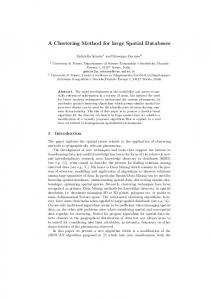
For each cell, geographical data is represented as humans perceive it in reality, that is, geometric (or physical) representation and thematic (or logical) representation. Geometric representation describes the geographical objects by means of the most appropriate physical entity (point, line or region), while thematic representation expresses the semantics of geographical objects (e.g., hydrography, vegetation, transportation network and so on), independently of their physical representation. The territory considered in this application covers 45 km2 from the zone of Canosa in Apulia (Italy). The examined area is segmented into square areal units of 1 Km2 each. Thus, the problem of recognizing spatial continuity of some morphological elements in the map is reformulated as the problem of grouping adjacent cells resulting in a morphologically homogeneous area, that is, a problem of clustering spatial objects according to the discrete spatial structure imposed by the relation of “adjacency” among cells. Since several geographical objects, possibly belonging to different layers (e.g., almond tree, olive tree, font, street, etc) are collected within each cell, we apply algorithms derived from geometrical and topological reasoning [9] to obtain cell descriptions in first-order formalism (see Figure 1). For this task, we consider descriptions including spatial descriptors encompassing geometrical properties (area, extension) and topological relations (regionT oRegion, lineT oLine, pointT oRegion) as well as non spatial descriptors (typeOf , subtypeOf ). The descriptor partOf is used to define the physical structure of a logical object. An example is: typeOf (f1 ) = f ont ∧ partOf (f1 , x1 ) = true, where f1 denotes a font which is physically represented by a point referred with the constant x1 . Each cell is here described by a conjunction of 946,866 ground selectors in average. To support some qualitative reasoning, a spatial background

knowledge (BK) is expressed in form of clauses. An example of BK we use in this task is: f ontT oP arcel(F ont, Culture) = Relation ← typeOf (F ont) = f ont, partOf (F ont, P oint) = true, typeOf (P arcel) = parcel, partOf (P arcel, Region) = true, pointT oRegion(P oint, Region) = Relation that allows to move from a physical to a logical level in describing the topological relation between the point that physically represents the font and the region that physically represents the culture and that are, respectively, referred to as the variables F ont and Culture. The specific goal of this study is to model the spatial continuity of some morphological environment (e.g. cultivation setting) within adjacent cells over the map. This means that each cluster covers a contiguous area over the map where it is possible to observe some specific environment that does not occur in adjacent cells not yet assigned to any cluster. The granularity of partitioning changes by varying homogeneity threshold (see Figure 2). In particular, when h − threshold = 0.95, CORSO clusters adjacent cells in five regions in 1821 secs. Running time refers to execution performed on an IBM notebook Mobile Intel(R) Pentium(R) with 4-M CPU 2.00GHz and 256 Mb of RAM. Theories associated to neighborhood merged in each cluster offer a description of the morphological environments they are modeling. In this study, we report a compact representation of such theories derived according to the intuition that merged neighborhoods share the same structure (i.e., same descriptors applied to same linked terms) possibly differing only in the corresponding function values. Theories associated to these neighborhoods can be synthetically represented as a single theory where each single function value is replaced by the super-set of them derived from starting theories when resulting theory is equivalent in coverage to the set of neighborhoods theories 2 . Consequently, clusters are described by: C1 : cluster(X1 ) = c1 ← containAlmondT ree(X1 , X2 ) = {true}, cultivationT oCulture(X2 , X3 ) = {outside}, areaCulture(X3 ) = [328..420112], f ontT oCulture(X4 , X3 ) = {outside}. C2 : cluster(X1 ) = c2 ← containAlmondT ree(X1 , X2 ) = {true}, cultivationT oCulture(X2 , X3 ) = {inside}, areaCulture(X3 ) = [13550 ..187525], areaCulture(X3 ) = [13550..187525], cultivationT oCulture(X2 , X4 ) ∈ {outside}. C3 : cluster(X1 ) = c3 ← containGrapevine(X1 , X2 ) = {true}, 2

In [8] the authors discuss details of the algorithm to merge a pair of first-order clauses H1 , H2 in a single clause H by preserving the equivalence of coverage, that is: (i) for each structured object o with H1 , H2 , BK |= o then H, BK |= o and vice-versa, (ii) for each structured object o with H1 , H2 , BK 6|= o then H, BK 6|= o and vice-versa, where BK is a set of first-order clauses.

0.8 1 1

2

3

0.85 4

5

1

C1

2

3

C1

0.9 4

5

1

2

C1

2

3

0.95 4

5

C2

1

2

C1

3 4

C2

3

4

5

C2 C3

C3

5 6 7

C2 C3

C4

C4

8

C5

9

Fig. 2. Spatial clusters detected on map data from the zone of Canosa by varying h − threshold value in {0.8,0.85,0.9,0.95}.

cultivationT oCulture(X2 , X3 ) = {inside}, areaCulture(X3 ) = [13550.. 212675], cultivationT oCulture(X2 , X4 ) = {outside}. cluster(X1 ) = c3 ← containGrapevine(X1 , X2 ) = {true}, cultivationT oCulture(X2 , X3 ) = {outside}, areaCulture(X3 ) = [150.. 212675], cultivationT oCulture(X2 , X4 ) = {outside, inside}. C4 : cluster(X1 ) = c4 ← containStreet(X1 , X2 ) = {true} streetT oCulture(X2 , X3 ) = {adjacent}, areaCulture(X3 ) = [620.. 230326], cultureT oCulture(X3 , X4 ) = {disjoint}. C5 : cluster(X1 ) = c5 ← containOliveT ree(X1 , X2 ) = true, cultivationT oCulture(X2 , X3 ) ∈ {outside}, areaCulture(X3 ) ∈ [620.. 144787], oliviT oP arcel(X2 , X4 ) = {outside}. Notice that each detected cluster effectively includes adjacent cells sharing a similar morphological environment, while separate clusters describe quite different environments. Spatial partitioning of CORSO is compared with the relational clustering performed with logical decision trees [1], which are able to manage relational structure of spatial objects but ignore relations imposed with discrete spatial structure. The empirical comparison with GDBSCAN was not possible since the system is not publicly available. Anyway, CORSO improves GDBSAN clustering that is not able to manage complex structure of spatial data. Conversely, the logical decision tree mined on the same data divides the territory under analysis in twenty different partitions where it is difficult to recognize the continuity of any morphology phenomenon.

4

Conclusions

In this paper an application of spatial clustering performed by CORSO in the topographic map interpretation has been illustrated. This study aims at detecting spatial continuity of some morphological environments (e.g., cultivation settings) over the topographic map of the Apulia region in Italy. The territory considered in this application covers 45 km2 from the zone of Canosa in Apulia. The examined area is segmented into square areal units of 1 Km2 each. Thus, the problem of recognizing spatial continuity of some morphological elements in the map is reformulated as the problem of grouping adjacent cells resulting in a morphologically homogeneous area, that is, a problem of clustering spatial objects according to the discrete spatial structure imposed by the relation of “adjacency” among cells. The multi-relational approach and the usage of first-order logic as representation and reasoning means is justified by the need to consider relations implicitly defined between spatial objects observed within each single areal unit (map cell) to be clustered. In this way, spatial relations and spatial reasoning rules (background knowledge) are easily represented by means of first-order logic clauses. Similarity among cells is then computed as degree of matching with respect to a common generalization (logical theory). Finally, relational constraints (adjacency among cells) forming the discrete structure arising in map data are represented as a graph and the concept of graph neighborhood is exploited to capture relational constraints embedded in the graph edges. As a consequence, only Apulian cells associated with (transitively) graph connected nodes can be clustered together according to judgment of similarity on relational descriptions representing their internal (spatial) structure. Results of clustering allow to detect the morphology of different cultivation settings in the area under analysis. As future work, we plan to investigate the possibility of assigning the same unit to multiple clusters and the definition some heuristic to be adopted when choosing the seed starting point in clustering detection.

5

Acknowledgment

The work presented in this paper is partial fulfillment of the research objective set by the ATENEO-2005 project on “Gestione dell’informazione non strutturata: modelli, metodi e architetture”.

References 1. L. De Raedt and H. Blockeel. Using Logical Decision Trees for Clustering. In S. Dˇzeroski and N. Lavraˇc, editors, International Workshop on Inductive Logic Programming, ILP 1997, volume LNAI 1297, pages 133–140. Springer-Verlag, 1997. 2. S. Dˇzeroski and N. Lavraˇc. Relational Data Mining. Springer-Verlag, 2001.

3. F. Esposito, D. Malerba, and G. Semeraro. Flexible Matching for Noisy Structural Descriptions. In International Joint Conference on Artificial Intelligence, IJCAI 1991, pages 658–664, 1991. 4. M. Ester, H.-P. Kriegel, J. Sander, and X. Xu. A Density-Based Algorithm for Discovering Clusters in Large Spatial Databases with Noise. In Knowledge Discovery in Databases, pages 226–231, 1996. 5. M. Kirsten and S. Wrobel. Relational Distance-Based Clustering. In D. Page, editor, International Conference on Inductive Logic Programming, ILP 1998, volume LNAI 1446, pages 261–270. Springer-Verlag, 1998. 6. K. Koperski. Progressive Refinement Approach to Spatial Data Mining. PhD thesis, Computing Science, Simon Fraser University, British Columbia, Canada, 1999. 7. D. Malerba. Learning Recursive Theories in the Normal ILP Setting. Fundamenta Informaticae, 57(1):39–77, 2003. 8. D. Malerba, A. Appice, A. Varlaro, and A. Lanza. Spatial Clustering of Structured Objects. In S. Kramer and B. Pfahringer, editors, International Conference on Inductive Logic Programming, ILP 2005, volume LNAI 3625, pages 227–245. Springer-Verlag, 2005. 9. D. Malerba, F. Esposito, A. Lanza, F. A. Lisi, and A. Appice. Empowering a GIS with Inductive Learning Capabilities: The Case of INGENS. Journal of Computers, Environment and Urban Systems, Elsevier Science, 27:265–281, 2003. 10. D. Mavroeidis and P. Flach. Improved Distances for Structured Data. In T. Horv´ ath and A. Yamamoto, editors, International Conference on Inductive Logic Programming, ILP 2003, volume LNAI 2835, pages 251–268. Springer-Verlag, 2003. 11. D. Patterson. Introduction to Artificial Intelligence and Expert Systems. PrenticeHall, 1991. 12. L. D. Raedt and S. Dzeroski. First-Order jk-Clausal Theories are PAC-Learnable. Artificial Intelligence, 70(1-2):375–392, 1994. 13. J. Sander, E. Martin, H.-P. Kriegel, and X. Xu. Density-Based Clustering in Spatial Databases: The Algorithm GDBSCAN and its Applications. Data Mining and Knowledge Discovery, 2(2):169–194, 1998. 14. T. Smith, P. Donna, M. Sudhakar, and A. Pankaj. KBGIS-II: A Knowledge-Based Geographic Information System. International Journal of Geographic Information Systems, 1(2):149–172, 1997. 15. G. Toussaint. Some Unsolved Problems on Proximity Graphs. In D. Dearholt and F. Harary, editors, First Workshop on Proximity Graphs, 1991. 16. X. Wang and H. J. Hamilton. DBRS: A Density-Based Spatial Clustering Method with Random Sampling. In Pacific-Asia Conference on Knowledge Discovery and Data Mining, PAKDD 2003, pages 563–575, 2003.