as a complementary source of information for urban planning applications, focusing ... available in social media applications is limited, with the exception of Twitter. ... geolocated tweets and the semantics of its content to interpret individual and ...
Spectral Clustering for Sensing Urban Land Use using Twitter Activity Vanessa Frias-Martineza, Enrique Frias-Martinezb a
College of Information Studies, University of Maryland, College Park, MD 20742 b Telefónica Research, Distrito Telefónica, 28050, Madrid, Spain
Abstract Individuals generate vast amounts of geolocated content through the use of mobile social media applications. In this context, Twitter has become an important sensor of the interactions between individuals and their environment. Building on this idea, this paper proposes the use of geolocated tweets as a complementary source of information for urban planning applications, focusing on the characterization of land use. The proposed technique uses unsupervised learning and automatically determines land uses in urban areas by clustering geographical regions with similar tweeting activity patterns. Three case studies are presented and validated for Manhattan (NYC), London (UK) and Madrid (Spain) using Twitter activity and land use information provided by the city planning departments. Results indicate that geolocated tweets can be used as a powerful data source for urban planning applications.
Keywords Urban computing, crowd behavior, land use detection, spectral clustering.
1. Introduction Urban planning is a process that focuses on the control and on the design of urban environments in order to increase the well being of citizens. An important concern in urban planning is the characterization of urban land use, such as residential, industrial or parks. How each part of an urban landscape is used, is mainly determined by zoning regulations. In the context of urban planning, urban zoning is defined as the designation of permitted uses of land based on mapped zones which separate one set of land uses from another (for example residential areas from industrial areas). One of the problems of zoning is to actually evaluate to which extent the areas are being used as required or planned, because the collection of data has to be done on site. Such information is usually gathered through direct observation or using questionnaires that attempt to capture how citizens interact with their urban environment. This traditional approach has some limitations such as the resiliency of citizens to provide answers or the cost of running questionnaires, which highly limits the frequency with which the information is captured. Alternative approaches such as GIS (Geographic Information Systems) (Yin et al., 2011) provide satellite imagery that might reveal some types of land use information through image processing techniques. However, such techniques fail to provide real time information as images are not captured frequently and the land uses that can be identified do not cover the variety of land uses present in a city. With the increasing capabilities of mobile devices, individuals leave behind footprints of their interaction with urban environments. In this context, cell phones have become one of the main sensors of human behavior, thanks, among others, to their growing penetration and wealth of social applications. As a result, new research areas, such as urban computing and smart cities, focus on improving the quality of life in an urban environment by understanding the city dynamics through the data provided by ubiquitous infrastructures and technologies. New data sources (including GPS, Bluetooth, WiFi hotspots, geo-tagged resources, cell phone traces, etc.) are becoming more relevant for urban planning applications such as transport planning (Frias-Martinez et al., 2012b), traffic estimation (Caceres et al., 2012) or social studies (Oloritun et al., 2013). In the literature we can find some approaches that use different pervasive infrastructures for the automatic identification of land uses such as GPS (Yuan et al. 2012), cell phone traces (Soto et al., 2011) or social media applications such as Foursquare (Noulas et al., 2011). In general these approaches tend to focus on specific land uses, on a specific city, and they lack a quantitative validation of the results. Also, GPS and cell phone traces are difficult to obtain due to privacy concerns, and in general, the location information available in social media applications is limited, with the exception of Twitter.
In this paper we propose to use Twitter geolocated data for the automatic identification of land uses. The proposed approach exclusively makes use of spatial (geo-tagged) and temporal (time-stamped) information of tweets, without accessing personal details or the content of the user-generated information. By doing so, it preserves privacy and can potentially be applied and/or complemented with any other mobile social media dataset with geolocation information. Our novel approach is designed to identify all possible land uses using spectral clustering, it is validated using real land use data provided by city planning departments and is tested in three different urban environments: Manhattan (NYC), London (UK) and Madrid (Spain).
2. Related Work Our work arises as a combination of two research areas mainly crowd modeling and urban computing for urban planning. Different authors have used a variety of user-generated content services for implementing crowd behavior models. Wakamiya et al. (2011) and Fujisaka et al. (2010) studied how to exploit geolocated tweets and the semantics of its content to interpret individual and crowd behavior i.e., how individuals and groups of people move across geographical areas. They propose models of aggregation and dispersion as a proxy to understand the bursty nature of human mobility. Similarly, Kinsella et al. (2011) used geolocated tweets, together with their content, to create geographical models at varying levels of granularity (from zip codes to countries). The authors use these models to predict both the location of the tweet and the user based on location changes. Recently, in the area of urban computing for urban planning we can find a variety of results using geolocated information to model land use. The approaches can be divided according to its source of information: (1) location-based social networks (LBSN) traces from Foursquare or Twitter; (2) call detail records (CDRs) from cell-phones; and (3) GPS traces. The three data sources represent a compromise between granularity and data generality: while GPS data has longitude-latitude information every couple of seconds for usually a very limited number of individuals (usually less than one hundred); CDRs have location information for millions of individuals at a tower level only when an interaction (call or SMS) takes place. LBSN offer an intermediate solution where location information is in the form of longitudelatitude for an intermediate number of individuals (usually hundred of thousands). Regarding LBSN, Noulas et al. (2011) have used the geolocated information provided by Foursquare to model crowd activity patterns in London and New York City using spectral clustering. For that purpose, the authors characterize the activity patterns identified by the clusters using the predefined Foursquare categories that give an indication of the type of check-in location (restaurants, academic, etc.). As such, this approach gives an approximated understanding of land use. Frias-Martinez et al. (2012), and Neuhaus (2011) presented preliminary results on using Twitter for characterizing urban landscapes. Both studies showed that geolocated tweets potentially contain enough information to identify some land uses, although with some limitations. In the case of Frias-Martinez et al. (2012) the main limitations arise due to the problems of using k-means as clustering technique to classify the terrain. In a related work Cranshaw et al. (2012) presents a new clustering model designed to study land use and social dynamics on a large scale using Foursquare. The results are validated with personal interviews that confirm the clusters identified. As for CDRs, Calabrese et al. (2011) used cell-phone records from Rome to study the relation between phone activity and commercial land uses using Principal Component Analysis (PCA) to identify the dominant pattern in each area. The results are qualitatively presented and validated and no land use information is actually used. A similar study was done by Ratti et al. (2006) in Milan. Soto et al. (2011) used the tower activity to characterize and cluster similar location patterns and implemented a qualitative evaluation of the results. Toole et al. (2012) also used activity patterns to cluster land uses using a random forest approach in Boston. GPS data sources are not as commonly used for land use purposes due to the privacy concerns. In general the traces available come from public transport infrastructure such as buses and taxis, which limits its generalization. Yuan et al. (2012) present an initial study using GPS traces from taxis to derive individual mobility and identify regions of different functions using a predefined map of the points of interest of Beijing, i.e. information of the city was used to derive land uses.
In general, the main limitations of the previous approaches are: (1) lack of a formal validation of the results using independent land use data; (2) the studies are presented just for one city, somehow limiting the potential generality of the proposed approach; (3) some data sources (mainly cell phone traces) have strong privacy limitations and (3) in some cases supervised approaches are used, which implies the need of having initial knowledge of the city to derive land uses. Our approach overcomes such limitations by using an unsupervised technique for land use classification that is based on an intermediate data source (both in the sense of number of individuals and privacy) such as Twitter. The approach is validated with external sources and its generality is tested using three cities as examples.
3. Sensing Urban Land Uses using Twitter The technique we propose for the automatic identification of urban land uses from geolocated tweets has two steps: (1) land segmentation and (2) land use detection. Note that the land uses (such as residential, industrial, parks, etc.) are not defined before hand but identified by the unsupervised learning technique.
3.1. Land Segmentation with Geolocated Data Given that we want to sense land uses in different urban regions, the first step consists on partitioning the land into different segments, which can then be characterized by its usage pattern. The partitioning of the area considered has to preserve the topological properties of the geolocated tweets, while respecting the actual shape of the geographical area under study. We approached this problem using Self-Organizing Maps (SOM) (Kohonen, 1990). SOM is a type of neural network trained using unsupervised learning that produces a two-dimensional representation of the training samples. It consists of nodes each one having a weight vector of the same dimension as the input data and a position in the two-dimensional space. Usually the initial weight of the vectors are random values and the initial arrangement of the nodes is a rectangular grid. The procedure for placing a vector from the input data onto the map is to find the node with the smallest distance metric to the data space vector, which in turn updates the weight and the position of the neuron. In our case, the input data are the latitude & longitude pairs that represent the geolocated tweets over a period of time for a specific urban area. As a result, we use a SOM to build a map that segments the urban land into geographical areas with different concentrations of tweets. Our SOM consists of a collection of N neurons organized in a rectangular grid [p, q], with N = p•q. Since we can choose any initial size [p, q] for the map, our method explores different map sizes and selects as the best land segmentation map the topology that minimizes the Davies-Bouldin clustering index (Davis et al., 1979). The DB index is used to evaluate clustering algorithms, where the validation of how well the clustering has been done is made using quantities and features inherent to the dataset. It is formally defined as: DB =
1 N
σi +σ j
N
∑ max d (w , w ) i =1
i≠ j
i
j
(1)
Where N is the number of clusters (neurons), wi and wj represent the position in the two dimensional space of the SOM neurons i and j, and σi and σj represent the standard deviation of the elements (geolocated tweets) included in each cluster. The DB index is chosen for land segmentation because the partition with minimum value will minimize the maximum sum of a pair of standard deviations σi and σj, i≠j and will maximize the distance between cluster representatives (neurons), ensuring that even the most disperse clusters concentrate its points (geolocated tweets) inside a compact cluster. As a result of the process, we obtain a map where each neuron represents a pointer to a region with a high density of tweets. Additionally, areas with larger concentrations of tweets will have larger numbers of neurons geographically located nearby. Finally, Voronoi tessellation (Aurenhammer, 1991) is applied over the location of the neurons in order to compute the land segments that each neuron represents. These land segments are used as the elements for the characterization of land use.
3.2. Unsupervised Learning for Detecting Urban Land Uses We characterize each land segment by its average tweeting activity which will then be used to identify common land uses. For each land segment s, a tweet-activity vector Xs representing the average tweeting behavior is built as: 1. An activity vector xs,n for land segment s is built for each day n =1, ..., d in the dataset. 2. Each day n in the activity vector contains 72 components xs,n (t), t = 1, ..., 72 where each one represents the number of tweets generated in land segment s during a 20-minute interval t in day n. 3. An average activity vector for each land segment s is computed for both weekdays Xs,wkd and weekends Xs,wkn, each one representing the average number of tweets (during the n days) in land segment s during the corresponding time period t, just considering weekdays (Monday through Friday) in the first case and weekends (Saturday and Sunday) in the second: d
∑x X s ,wkd (t ) =
s ,n ( t )
n =1
, t = 1,...,72, n ∈ weekday
n
(2)
d
∑x X s ,wkn (t ) =
s ,n ( t )
n =1
, t = 1,...,72, n ∈ weekendday
n
4. The final activity vector is represented as the concatenation of weekday and weekend average activity vectors Xs = {Xs,wkd,Xs,wkn} and is normalized as: _
X s (t ) =
X s (t ) 72
∑X
72
s , wkd
(t ) + ∑ X s ,wkn (t )
t =1
(3)
t =1
After this process, each land segment s is represented by a unique activity vector Xs with 144 elements representing the average weekday and weekend tweeting activity computed in 20-minute timeslots. These activity vectors are used to automatically identify and characterize urban land uses using clustering. We posit that land use can be derived from a careful analysis of the tweeting behaviors in each cluster, based on its activity vector as well as on its physical layout in the city. From the variety of clustering techniques available that can be potentially applied to our land segmentation problem (k-means, hierarchical methods, decision trees, Fuzzy Clustering, etc.) we have selected spectral clustering (Shi et al., 2000; Von Luxburg 2007). Spectral clustering has become increasingly popular due to its advantages, including that no assumptions about the form of the clusters is made (as opposed to k-means for example); that is able to manage large dimensional datasets by using dimensionality reduction; that it is easy to implement using standard linear algebra; and that it obtains good clustering results with a low computational cost. Also it has already been used with success in related urban computing applications, such as in Noulas et al. (2011) to divide communities. Spectral clustering first requires the number k of clusters to construct, and a similarity matrix S that represents the pair wise similarities si,j=s(Xi, Xj) of all elements. In our context Xi and Xj represent the tweeting activity of each one of the land segments previously obtained. The similarity si,j of two vectors Xi and Xj is measured as the cosine similarity: si , j = s ( X i , X j ) =
Xi X j Xi X j
(4)
Cosine similarity values range from -1 implying exactly opposite to 1 meaning exactly the same. The algorithm treats the data clustering problem as a graph partitioning problem, and as such, the first step is to build a similarity graph G = (V, E). Each vertex vi represents a data point xi and two vertices are connected by an edge ei,j if the similarity si,j is positive; si,j>0. Two matrices are then created, a weighted adjacency matrix W (with the values of si,j>0) and a degree matrix D. In this context, clustering can be
reformulated as finding a partition of D such that the edges between different groups have very low weights and the edges within a group have high weights as defined in W. The simplest version of the algorithm performs first a dimensionality reduction and then applies a clustering algorithm, typically k-means. It starts by using the degree matrix D and the weight matrix W to construct a Laplacian matrix L as (Chung, 1997; Mohar 1997): L = D −W
(5)
After that, a matrix U is built containing as columns the first k eigenvectors of L. Then, each one of the rows of U is clustered into k clusters using k-means (Hartigan et al., 1979), which outputs the clusters identified with its corresponding elements. Regarding the number of clusters k, which has to be given as an input, the eigengap detection technique is specially suited (Luxburg, 2007). With this approach the number of clusters k is defined by the rank of the eigenvalues where there is the largest difference in the value of the eigenvalues of the Laplacian matrix arranged in increasing order. By applying spectral clustering to our problem, we obtain as output k clusters each one containing the set of activity vectors of the land segments included in each clusters. In order to analyze the type of land associated to each cluster, we compute an average activity vector that represents the tweeting activity of each cluster. Finally, we hypothesize the land use for each cluster based on its tweeting activity and its distribution across the urban environment under study.
4. Evaluation of Land Uses We present an evaluation of our land use detection method for three metropolitan areas: Manhattan (NYC), London (UK) and Madrid (Spain). We have selected these three cities because they show different densities of Twitter activity computed as the number of daily tweets per square kilometer in the urban perimeter considered: Manhattan has the highest Twitter density (84.13 tweets/km2) followed by London with about half of that (42.51 tweets/km2) and Madrid with a density of 10.88 tweets per square kilometer. As such, these three cities represent different cultural and behavioral Twitter attitudes useful to evaluate the limits of our approach. The objective of this evaluation is twofold: (1) to analyze to which extent the land use identification algorithm detects different types of land uses and (2) to understand the impact of the density of tweets on the accuracy of the method proposed. For that purpose we apply the algorithm on Twitter datasets of each one of the three cities considered and draw hypothesis regarding land uses based on both tweeting activity and location. To validate our results, we contrast our clusters and land uses hypotheses against real land use information collected by the corresponding city planning department.
4.1 Twitter Datasets Twitter users are allowed to tag tweets with their current geospatial location. Specifically, users can set their geographical location by specifying a city or region or by allowing Twitter to track their GPS longitude and latitude coordinates. When a new tweet is produced, Twitter records the geographical information of the user at that moment, along with a variety of other metadata. Given that we want to model land use within an urban environment, we require highly granular geolocations. Thus, we only collect tweets whose location is automatically recorded by Twitter through the GPS and not self-reported by the user. We used the Twitter Streaming API (Twitter, 2013) to gather geolocalized tweets in near real-time. The streaming API enables a high-throughput stream to be established with Twitter by which a large volume of public statuses of tweets can be gathered. Specifically, the Twitter steaming API provides a sample of all tweet public statuses, currently about one percent of the full Firehose set of tweets. Our final Twitter dataset consists of 49 days (seven weeks) of geolocated tweets worldwide from October 25th to December 12th, 2010. The geographical area for London is defined by the area defined by what would have been Ringway 1*. As for Madrid, we roughly consider the urban area comprised within the M − 30 highway. *
http://www.cbrd.co.uk/histories/ringways/map/google-download.shtml
4.2 Land Segmentation and Land Use Clustering Our method trains a SOM with the set of geolocated tweets to divide the urban area under study into different land segments s characterized by their tweeting activity vector Xs. Given the different geographies of the cities under study, we evaluated N in the range N = [10,..., 300] with N defined as: N = p ⋅ q with p, q > 1 and p, q ∈
(6)
The values of p and q define the number of neurons considered in each axis: p in the north-south axis and q in the east-west axis (we leave out the cases where N is a prime number). To adjust the neurons to the shape of each city, we only consider cases in which p > q for Manhattan and Madrid and p < q for London (Manhattan and Madrid have a longer north-south axis and London has a longer east-west axis). For example, in Manhattan N = 10 would define an initial grid with p = 5 and q = 2 and N = 12 would generate (p = 6, q = 2) and (p = 4, q = 3). Due to the randomized nature of the SOM training stage, 100 SOMs are trained for each city and each pair (p, q) with N = p · q є [10,..., 300] and their average DB index is computed. The minimum DB index was associated to N = 64 for Manhattan with p = 16 and q = 4; N = 168 for London with p = 12 and q = 14; and finally N = 91 for Madrid with p = 7 and q = 13. As an example, Figure 1 shows the land segmentation for Manhattan. We observe that the Midtown area, where the best part of the tweets are geolocated (as shown in Figure 1(a)), shows a high density of neurons; whereas the north of Manhattan, with a scarce number of tweets, has a reduced number of neurons. Finally, the land segmentation is computed by applying Voronoi tessellation (Aurenhammer, 1991) to each SOM centroid in the two-dimensional space as shown in Figure 1(c). Notice that areas with larger polygons represent areas with reduced Twitter activity. Each one of the land segments identified in Manhattan, London and Madrid is characterized by its Twitter activity vector Xs which has 144 components; the first 72 describe the tweeting activity during an average weekday and the last 72 the activity during and average weekend day. Note that the number of Xs vectors for each city is given by the optimal number of SOM neurons identified in each case (64 for Manhattan, 168 for London and 91 for Madrid). Our method uses the set of Xs vectors to identify different land uses for each city identifying clusters of similar normalized activity using spectral clustering; i.e., the similarity graph G is build in each case with the set of corresponding Xs vectors. In order to identify the number of clusters k, we followed the eigenvector detection approach. As a result, the best number of land segment clusters is k = 4 for Manhattan and Madrid, and k = 5 for London. Table 1 summarizes for each city the parameters of each urban environment. In order to understand the types of land uses identified by these clusters, we analyze the class representatives for each cluster together with its geographical distribution over the city map. A combined analysis can be used to provide a hypothesis about the potential types of land uses. Figure 2 presents the class representatives for each one of the clusters identified across the three cities. Each representative (behavioral signature) is computed as the average number of hourly tweets and is normalized per cluster and per city. For analytical purposes, we group the signatures across cities by Euclidean similarity. We hypothesize that signatures that share similar shapes across cities represent comparable land use types. We observe that the activity vectors in Cluster 1 are generally characterized by a larger tweeting activity during weekdays than weekends (see Figure 2(a)). During weekdays the highest tweeting activity is reached at around 9:30PM, 13:00PM and 8:30PM for Manhattan, which might be associated to the times at which people typically get to work, go for lunch, and leave work. The city of London shows similar peaks but slightly shifted in time. In the case of Madrid, the signature is shifted even more, suggesting that working hours might happen a little bit later during the day. The peak of the tweeting activity during the weekends is reduced by approximately 40% when compared to weekdays. In terms of geolocation of the clusters, these cover, among others, areas like Battery Park or Wall Street in Manhattan (see Figure 3), the City and Canary Warf in London (see Figure 5) and the surroundings of Castellana and the area of AZCA in Madrid (see Figure 4), all areas heavily associated with business/office activities. For these reasons, we hypothesize that the geographical area covered by this cluster represents Business areas in Manhattan, London and Madrid.
Cluster 2 shows a large difference between weekend and weekday activity, in fact, the signature is almost doubled in volume (see Figure 2(b)). During weekends, tweeting activity increases until the afternoon, and constantly decreases after that. Geographically, these clusters cover regions like Central Park and nearby museums in Manhattan (see Figure 3), Hyde Park or Regents Park in London (see Figure 5) and El Retiro Park and Casa de Campo Recreational Park in Madrid (see Figure 4). Also included are heavily touristic areas, like Sol and the Flea Market of El Rastro in Madrid, or the London Eye, Buckingham Palace and Covent Garden in London. Thus, we hypothesize that this cluster can be associated to Leisure or Weekend activities since users are active mostly during the weekends. However, we believe that it does not represent weekend nightlife since the tweeting activity highly decreases after 16:00PM during the weekends. On the other hand, Cluster 3 is associated to very large activity peaks at night (see Figure 2(c)). These peaks happen at around 20:00-21:00PM during weekdays and between 00:00-06:00AM during the weekends. We observe that the peaks happen earlier in London and Manhattan while a little bit later in Madrid suggesting that nightlife might continue until late hours in this city. Studying the physical layout of these clusters on the city maps, we observe that they cover areas like the East Village in Manhattan; the West End in London and Malasaña/Chueca and Alonso Martinez in Madrid (see Figure 4), areas associated with restaurants, pubs and discos. All these elements suggest that this cluster might represent nightlife activities. Cluster 4 shows a signature evenly divided between weekends and weekdays, where, during weekdays, there is a peak of activity in the afternoon between 6pm and 8pm depending on the urban area considered (6pm for Manhattan and London and 8pm for Madrid). Activity during weekends is of the same magnitude as in weekdays (see Figure 2(d)). This is the most important cluster considering the geographical area covered and the number of clusters included. The geographic layout of the clusters cover heavily residential areas in all cities: in Manhattan the limits of the island and in Madrid and London the outskirts of the areas considered. In Figures 3, 4 and 5, the areas include with this cluster are the ones not marked with any color. Our hypothesis for this type of signature is that it represents residential land use with citizens tweeting from home at any time during the weekends and after working hours during the week. Finally, Cluster 5 is only identified for London (see Figure 2(e)). Its signature is characterized by a reduced activity during the weekends. The weekdays show a peak in activity very early, at around 10am, after which a steady decrease happens showing little activity during the rest of the day. Looking at the physical layout, these clusters cover areas in the east and south of the city, like the area around Battersea Station and the Olympic Park. As a result of that, we hypothesize that this cluster represents Industrial land use (see Figure 5). Finally, it is important to clarify that we have only focused on identifying the main land use of each cluster (although there might be other minor ones), since this is the way urban planners typically compute land use maps.
4.3 Land Use Validation In order to validate our land use hypotheses, we compare the evaluation results against official land use data released by the NYC Department of City Planning and the NYC Department of Parks & Recreation through the NYC Open Data Initiative (NYC, 2013); against the ward profiles released by the London Datastore Open Data Initiative (London, 2013) and against the district land use information computed by the Urban Planning Department in Madrid’s City Hall (Madrid, 2013). These catalogs are produced by city agencies typically through a combination of on-site inspections, interviews and questionnaires. The NYC Department of City Planning considers four main land use types: (1) residential, (2) commercial, (3) industrial and (4) parks & recreation (see Figure 6(a) for details). On the other hand, the information provided by the London Datastore considers three types of wards: (1) domestic buildings, which we associate to residential areas, (2) non-domestic buildings, which we pair up with business and industrial land use wards and (3) green spaces and paths. Finally, the information provided by the Urban City Planning Department in Madrid provides land use information at a district level and considers four types: (1) residential areas with different density levels (which we group), (2) industrial, (3) services(commercial & business) and (4) green spaces, as can be seen in Figure 6(b).
To understand how well the clusters we have identified using Twitter activity represent the official land use areas, we evaluate the percentage of overlapping that exists between the physical layout of the clusters and the official land use map for each city under study. Such analysis will give us an understanding of the accuracy of our approach to identify land uses as well as of the impact that the Twitter density might have on the quality of the results. It is important to highlight that the percentage of overlapping is an approximate measure to validate land use identification given that both maps have different granularities: our cluster maps represent land segment clusters based on Voronoi and tweet density whereas the official land use maps show data at a block, ward or district level, depending on the city. Table 2 shows the percentages of overlap between the official land use maps for each city (rows) and our land use hypotheses (columns). Each element (i, j) in the tables represents the percentage of the official land use region that is covered by one of our land use clusters i.e., Business, Residential, Nightlife, Leisure and Industrial. Note that in the case of Manhattan our Voronoi approximation to the island does not precisely cover all Manhattan land due to its irregularities, and as a result the percentage does not exactly sum up to 100%. Comparing our results across cities, we observe that Manhattan shows the highest percentages of official areas covered by our clusters, whereas London and Madrid share lower accuracies in terms of land use identification. It appears that the higher tweeting density that Manhattan has (84.13/km2) has, as expected, a positive impact on the quality of land use identification. The official Commercial and Business land uses in the three cities are identified quite well by our business cluster with area coverage between 61% − 81%. London is a special case in which the official non-residential land use is partially identified by our business cluster (61%) but also by our industrial cluster (25%). Similarly, the official Residential/Domestic buildings land use has a high overlap with our residential cluster with coverage between 56% and 68% of the official areas. However, we observe a generalized trend across the three cities whereby around a 20% of the official residential area is also covered by our nightlife clusters, probably highlighting residential areas with high densities of bars and restaurants. This is in fact common in areas like the East Village in New York, Chelsea in London or Chueca in Madrid. While in London we are able to detect Industrial land use, and compare it to the official non-residential land use, the official Industry land use, present in Manhattan and in Madrid, goes undetected. We consider that the main reason for that is that in both cases, within the area of the city considered, industrial land is minimum (less than 3% of the total area in Madrid and less than 8% in Manhattan), and as a result they are included in larger Voronoi elements that has a different stronger land use. In fact, most of the official industrial land use is subsumed by our residential cluster in the case of Manhattan whereas in Madrid it is mostly covered by our business cluster. This might indicate that workers in the industrial areas are not using Twitter as much as people that live and/or work in that area, and as a result our technique captures the main land use, i.e. the official land use goes undetected due to lack of activity. Finally, the official Parks & Recreation and Greenspace & Paths land use is identified by our leisure cluster with overlaps between 71% and 81% of the official land use maps. On the other hand, our method identified a Nightlife cluster that has no counterpart in any of the official land uses. Nightlife clusters mostly overlap with the official Residential land use. However, we wanted to understand whether the cluster is incorrect or whether it is modeling a different type of land use not accounted for by the city halls. For the particular case of Manhattan, we identified the number of noise complaints per community district made to the 311 on-line service during 2010 (see Figure 6(c)). Given that the community districts have much lower granularity than our land use clusters, we computed the percentage of the Nightlife cluster that is included within the districts with the highest number of complaints, which corresponds to an 82% of overlap. Thus, it is fair to say that the Nightlife cluster detected by our method identifies a Nightlife land use that could be of interest for city halls to model potential areas of noise complaints. We did not find such validation information for London and Madrid. Our evaluation and validation for three different cities with varied physical layouts shows two important results. First, our methodology constitutes a good complement to model and understand in an affordable and near real-time manner land uses in urban environments. In fact, we have shown that residential, commercial and parks & recreation areas are well identified with coverage above 70%. Also, our approach is able to identify a land use, nightlife activity, not being considered up to now by city halls. This has implications from a planning perspective as these areas usually cause noise and security problems and can move over time.
Second, Twitter density appears to have a reduced impact on the accuracy of our land use identification approach. As reported, coverage percentages of Manhattan, with a density of 84.13 tweets/km2 are slightly higher than those for London and Madrid with densities of and 42.51 tweets/km2 and 10.88 tweets/km2, respectively. However, although the accuracy of the land use detection is slightly lower, the results still offer significant information for land urban planners. The reason for the reduced impact is probably that as a result of normalizing the activity vectors Xs = {Xs,wkd,Xs,wkn}, clustering groups elements that have the same shape and not the same activity which limits the impact of the density of tweets on the results.
5. Conclusions With the deployment of pervasive infrastructures and the increasing use of geolocated user-generated content, urban planning will have a relevant and real-time source of information for characterizing urban dynamics. In this paper we have presented and validated an unsupervised approach for identifying land uses using location-based social media in Manhattan, London and Madrid. The implementation has been done with Twitter, although the same technique can potentially be used with other social media, provided it has geolocated information. The results have shown that geolocated tweets can constitute a good complement for urban planners to model and understand traditional land uses (like industrial or residential) and identify new ones (like nigh activities) in an affordable and near real-time manner. We will continue to address this challenge and expand our methodology by combining geolocated information with the content of tweets.
References Aurenhammer, F., 1991. Voronoi Diagrams – A Survey of a Fundamental Geometric Data Structure. ACM Computing Surveys, 23(3):345–405. Caceres, N., Romero, L. M., Benitez, F. G., & Del Castillo, J. M., 2012. Traffic flow estimation models using cellular phone data. Intelligent Transportation Systems, IEEE Transactions on, 13(3), 1430-1441. Calabrese, F., Colonna, M., Lovisolo, P., Parata, D., & Ratti, C., 2011. Real-time urban monitoring using cell phones: A case study in Rome. Intelligent Transportation Systems, IEEE Transactions on, 12(1), 141-151. Chung, F. R., 1997. Spectral graph theory (Vol. 92). American Mathematical Soc.. Cranshaw, J., Schwartz, R., Hong, J., Sadeh, N., 2012. The livehoods project: Utilizing social media to understand the dynamics of a city. In: AAAI Conf. on Weblogs and Social Media(ICWSM). Davies, D.L., Bouldin, D.W., 1979. A Cluster Separation Measure. IEEE Transactions on Pattern Analysis and Machine Intelligence, 1(2):224–227. Frias-Martinez, V., Soto, V., Hohwald, H., Frias-Martinez, E., 2012. Characterizing Urban Landscapes using Geolocated Tweets. In: Int. Conference on Social Computing (SocialCom), Amsterdam, The Nederlands, 239-248. Frias-Martinez, V., Soguero, C., & Frias-Martinez, E., 2012b. Estimation of urban commuting patterns using cellphone network data. In Proceedings of the ACM SIGKDD International Workshop on Urban Computing (pp. 916). ACM. Fujisaka, T., Lee, R., Sumiya, K., 2010. Exploring urban characteristics using movement history of mass mobile microbloggers. In: Proc.11th ACM Workshop on Mobile Computing Systems & Applications, 13–18. Hartigan, J. A., Wong, M. A., 1979. Algorithm AS 136: A k-means clustering algorithm. Applied statistics, 100-108. Kinsella, S., Murdock, V., O´Hare, N., 2011. I am eating a sandwich in Glasgow: modelling locations with tweets. In: Proc. of the 3rd Workshop on Search and Mining User-generated Contents, 61-68. Kohonen. T., 1990. The Self-Organizing Map. Proceedings of the IEEE, 78(9):1464–1480. London. London open data, 2013. http://data.london.gov.uk/visualisations/atlas/ward-profiles-summary/atlas.htm. Luxburg, U., 2007. A tutorial on spectral clustering. Statistics and Computing, 17(4), 395-416. Madrid. Madrid open data. 2013. http://www.madrid.org/cartografia/idem/html/web/index.htm. Mohar, B., 1997. Some applications of Laplace eigenvalues of graphs (pp. 225-275). Springer Netherlands. Neuhaus, F., 2011. New city landscape – Mapping urban Twitter usage. Technoetic 9(1), 31-48.
Noulas, A., Scellato, S., Mascolo, C., Pontil, M., 2011. Exploiting semantic annotations for clustering geographic areas and users in location-based social networks. In: 3rd Workshop Social Mobile Web. NYC. NYC open data, 2013. https://nycopendata.socrata.com/. Oloritun, R. O., Madan, A., Pentland, A., & Khayal, I., 2013. Identifying Close Friendships in a Sensed Social Network. Procedia-Social and Behavioral Sciences, 79, 18-26. Ratti, C., Williams, S., Frenchman, D., & Pulselli, R. M., 2006. Mobile landscapes: using location data from cell phones for urban analysis. Environment and Planning B Planning and Design, 33(5), 727. Shi, J., Malik, J., 2000. Normalized cuts and image segmentation. Pattern Analysis and Machine Intelligence, IEEE Transactions on, 22(8):888–905. Soto, V., & Frias-Martinez, E., 2011. Robust land use characterization of urban landscapes using cell phone data. In 1st Workshop on Pervasive Urban Applications, in conjunction with 9th Int. Conf. Pervasive Computing. Toole, J. L., Ulm, M., González, M. C., & Bauer, D., 2012. Inferring land use from mobile phone activity. In Proceedings of the ACM SIGKDD International Workshop on Urban Computing (pp. 1-8). ACM. Twitter. Open twitter streaming api, 2013. https://dev.twitter.com/docs/streaming-api. Von Luxburg, U. (2007). A tutorial on spectral clustering. Statistics and computing, 17(4), 395-416. Wakamiya, S., Lee, R., Sumiya, K., 2011. Urban area characterization based on semantics of crowd activities in twitter. In GeoSpatial Semantics, volume 6631 of Lecture Notes in Computer Science, pages 108–123. Springer Berlin / Heidelberg. Yin, J., Yin, Z., Zhong, H., Xu, S., Hu, X., Wang, J., & Wu, J., 2011. Monitoring urban expansion and land use/land cover changes of Shanghai metropolitan area during the transitional economy (1979–2009) in China. Environmental monitoring and assessment, 177(1-4), 609-621. Yuan, J., Zheng, Y., & Xie, X., 2012. Discovering regions of different functions in a city using human mobility and POIs. In Proceedings of the 18th ACM SIGKDD international conference on Knowledge discovery and data mining (pp. 186-194). ACM.
(a)
(b)
(c)
Figure 1: Land segmentation for Manhattan: (a) data points, i.e. geolocated tweets; (b) centers of activity computed with SOM, i.e. final location of the neurons after training; and (c) Voronoi tessellation.
(a) Cluster Type 1: Business
(b) Cluster Type 2: Leisure /Weekend
(c) Cluster Type 3: Nightlife
(d) Cluster Type 4: Residential
(e) Cluster Type 5: Industrial Figure 2: Tweeting activity signatures per cluster for Manhattan (black), London (blue) and Madrid (red). The Y axis represents the normalized tweeting activity and the X axis two 24-hour (0-23:59) periods, the first one for an average weekday and the second one for an average weekend.
Figure 3: Physical layout of business, nightlife and leisure clusters in Manhattan. Areas not marked with any color indicate residential land use.
Figure 4: Physical layout of business, nightlife and leisure clusters in Madrid. Areas not marked with any color indicate residential land use.
Figure 5: Physical layout of business, nightlife, leisure and industrial clusters in London. Areas not marked with any color indicate residential land use.
(a) Manhattan official land uses: Commercial, Residential, Industrial and Parks&Leisure official.
(b) Madrid official land uses: Commercial& Business, Residential (different densities considered), Industrial and Greenspaces.
(c) Manhattan: Districts with Noise Complaints (NYC 311Service, red represents the highest number of complaints)
Figure 6: Official Land Use Maps for Manhattan (a) and Madrid (b) and (c) Number of noise complaints in Manhattan per district.
Area Considered 54 km2 123.3 km2 93.6 km2
Manhattan London Madrid
tweets/km2 84.13 42.51 10.88
Number of Neurons (N) 64 168 91
Distribution (p, q) p=16, q=4 p=12, q=14 p=7, q=13
Number of Land Uses (k) 4 5 4
Table 1: Main parameters for the characterization of each urban environment.
Official Land Use
Twitter Land Use Business
Residential
Nightlife
Leisure& Weekend
Industrial
London Non-domestic buildings 1t1Domestic Buildings Greenspace & Paths
61% 9% 8%
9% 56% 11%
3% 23% 7%
2% 6% 72%
25% 6% 2%
81% 7% 13% 6%
12% 68% 77% 7%
3% 19% 0% 6%
2% 4% 6% 81%
-
69% 11% 58% 7%
25% 61% 33% 16%
4% 18% 3% 6%
2% 10% 6% 71%
-
Manhattan Commercial Residential Industry Park & Recreation
Madrid Commercial & Business Residential Industry Greenspace
Table 2: Percentage of overlap between official land uses and Twitter land uses for Manhattan, London and Madrid.