2016 8th Computer Science and Electronic Engineering Conference (CEEC)
University of Essex, UK
Spectral Clustering Using the kNN-MST Similarity Graph Patrick Veenstra
Colin Cooper
Steve Phelps
Department of Informatics King’s College London Strand, London WC2R 2LS Email:
[email protected]
Department of Informatics King’s College London Strand, London WC2R 2LS Email:
[email protected]
Department of Informatics King’s College London Strand, London WC2R 2LS Email:
[email protected]
Abstract—Spectral clustering is a technique that uses the spectrum of a similarity graph to cluster data. Part of this procedure involves calculating the similarity between data points and creating a similarity graph from the resulting similarity matrix. This is ordinarily achieved by creating a k-nearest neighbour (kNN) graph. In this paper, we show the benefits of using a different similarity graph, namely the union of the kNN graph and the minimum spanning tree of the negated similarity matrix (kNN-MST). We show that this has some distinct advantages on both synthetic and real datasets. Specifically, the clustering accuracy of kNN-MST is less dependent on the choice of k than kNN is.
I. I NTRODUCTION Clustering is an important task in data exploration, with the aim being to group objects or observations in such a way that objects within the same group are broadly more similar to one another than they are to objects in other groups. Spectral clustering is a group of methods that use the spectrum of a similarity matrix, or a matrix derived from it, to cluster the data. One of the most basic variants is described as follows [1]. Given a matrix A ∈ Rm×n containing m observations with n features, a similarity between each pair i, j of observations can be computed using a similarity measure. One such measure in common use is the Gaussian similarity measure [2]. Given that xi is the i-th row of A, then the similarity between observations i and j is defined as: � � �xi − xj �2 (1) s(xi , xj ) = exp − 2σ 2
Where xi , xj ∈ Rn and �xi − xj � is the Euclidean distance between the two vectors and σ controls the width of the neighbourhoods [1]. There are various suggestions for choosing σ; a common choice is for σ to be the standard deviation of the observations �xi − xj �, which is what we will use in this paper. [3] In this way, the similarity between every pair i, j can be computed and a similarity matrix S can be constructed where Sij = s(xi , xj ). At this point, a similarity graph G is constructed. The graph G = (V, E) consists of a finite set V = {v1 . . . vn } of vertices and a finite set E of edges, where each edge is an unordered pair connecting two vertices in V . There are many ways in which to construct G. The aim is to construct a graph such
978-1-5090-2050-8/16/$31.00 ©2016 IEEE
that similar observations are closely connected and dissimilar observations are not. The clustering problem then becomes that of finding a partition of the graph G such that edges between different clusters have low weight (low similarity). One such similarity graph, and the one we focus on in this paper, is the k-nearest neighbour graph. For each i ∈ {1 . . . m}, the edges to the k observations with highest similarities to i in S are added to the graph. Due to useful spectral properties exhibited by the graph Laplacian [4], the spectrum is calculated for the Laplacian of the similarity graph, rather than on the similarity graph itself. Given that W be the adjacency matrix of G, then the unnormalised Laplacian Lun of W is: Lun = D − W
(2)
Where D is the diagonal matrix containing the degree of each vertex on its diagonal. The degree di of vertex i is the sum of the entries in the i-th row of W. If we wish to divide the data into l clusters, we now compute the first l eigenvectors of Lun , that is, the l eigenvectors corresponding to the l lowest eigenvalues. Let U ∈ Rm×l be the matrix containing the first l eigenvectors (u1 , ..., ul ) as columns. Let yi be the i-th row of U. The clusters are then found by using k-means clustering to cluster the points (yi )i=1,...,m ∈ Rl into clusters C1 , ..., Cl . There are many varieties of spectral clustering, most notably, by changing the type of Laplacian used. Using the unnormalised Laplacian Lun as described above is known as unnormalised spectral clustering. Two popular variations that are based around normalised Laplacians are the normalised random walk spectral clustering [5] and normalised symmetric spectral clustering [2] that use Lrw and Lsym respectively: Lrw = D−1 Lun
(3)
Lsym = D−1/2 Lun D−1/2
(4)
We will use Lsym throughout this paper. The focus of this paper is the step of creating the similarity graph. We will show that by including the minimum spanning tree (MST)
222
2016 8th Computer Science and Electronic Engineering Conference (CEEC)
of the negated similarity matrix into the k-nearest neighbour (kNN) similarity graph, the quality of the clusters detected by the spectral clustering procedure becomes less sensitive to the choice of k. A. Sensitivity to k When using kNN as the similarity graph in spectral clustering, the choice of k can have a significant influence on the accuracy of the detected clusters when compared to the ground truth. A key reason for this is the connectivity of the similarity graph. The following is true for the spectrum of all three Laplacians discussed, Lun , Lsym and Lrw . If a similarity graph G has c disconnected components, then the multiplicity of the eigenvalue 0 is equal to the number of disconnected components c. The first c eigenvectors work to separate those components. Therefore, if one were to look for l clusters, but c > l, then this results in less accurate clustering as only the first l eigenvectors are used in the spectral clustering algorithm. Therefore, it is important to choose a good value for k to ensure at the very least, that the kNN similarity graph is connected. In general, the optimal choice of k does not have a closed form solution. But due to asymptotic connectivity results, it is common to choose �log n� for k [6]. The key result in this paper is to make the search for the optimal k less important. By adding the minimum spanning tree to the kNN similarity graph, connectivity is guaranteed. There will be no disconnected components. In this paper we will show empirically that doing this leads to more consistent results. In section II we introduce the kNN-MST method and in section III we demonstrate our argument on the well known Iris dataset from Fisher. We then look at both synthetic and real datasets in section IV. The conclusion is outlined in section V. II. M INIMUM S PANNING T REES AND K -N EAREST N EIGHBOURS In this paper we show that spectral clustering on a similarity graph consisting of the union of 1) the kNN similarity graph [7] and 2) the minimum spanning tree [8] of the negated complete similarity matrix, tends to perform better than kNN. Given a similarity matrix S, we can produce the adjacency matrix W(k) corresponding to the k-nearest neighbour similarity graph � with a simple procedure. Let � (p) xi , p ∈ {1 . . . (n − 1)} be the sequence of the n − 1 neighbours of i ordered from the closest to the furthest neighbour; from the most similar to the least similar. That (p) is, xi is the index of the p-th most similar neighbour to i. We can then define the matrix W(k) as follows: � (1) (k) Sij if j ∈ {xi , .., xi } (k) Wij = 0 otherwise W(k) is the adjacency matrix corresponding to the kNN similarity graph for S.
University of Essex, UK
A minimum spanning tree (MST) is a tree (connected undirected graph with no cycles) that spans a graph such that the sum of edge weights is less than or equal to that of any other tree of the graph. If we treat the negated complete similarity matrix −S as an adjacency matrix for a graph, then that graph G will be a complete graph. Let G(M ST ) be the MST for that graph, and let W(M ST ) be the adjacency matrix of G(M ST ) . Note that the minimum spanning tree was taken for the negated similarity matrix so that the minimum spanning tree contains the edges representing the highest similarities. The second MST can be found by removing from −S the elements that are part of the MST of −S, and then finding the minimum spanning tree for that modified version of −S. We define kMST to be the similarity graph defined as the union of the first k minimum spanning trees of −S. We will look at kMST in our results to demonstrate that the use of the kNN-MST similarity graph leads to more accurate clusters both due to the MST portion and the kNN portion. That is, kNN-MST performs better than either kNN or kMST individually. Let kNN-MST be the similarity graph created by taking the union of the first MST of the negated complete similarity matrix and the kNN similarity graph. That is, let the kNNMST similarity graph be defined as G(kN N M ST ) = (V, E), where V is the set of n vertices and E is defined as: E(G(kN N M ST ) ) = E(G(M ST ) ) ∪ E(G(kN N ) ) Let W(kN N M ST ) be the adjacency matrix of G(kN N M ST ) . In the next sections, we will show that the use of G(kN N M ST ) as a similarity graph in spectral clustering has advantages over using G(kN N ) . III. A N E XAMPLE USING F ISHER ’ S I RIS DATASET Fisher’s Iris Flower dataset consists of 150 observations with 4 features [9]. Each of the 150 observations is classified as being part of one of three species of Iris, namely Iris setosa, Iris Virginica and Iris versicolor. We will use the adjusted Rand index to quantify the accuracy of the clusters determined by the spectral clustering algorithms [10]. A value of 1 indicates perfect agreement between the ground truth clusters and the clusters identified by the clustering algorithm. A value close to 0 indicates that any agreement is mostly due to chance. Figure 1 shows the adjusted Rand index of the clusters identified by spectral clustering with the use of kNN, kMST and kNN-MST as the similarity graphs for the Iris dataset. The key point is that while equally good clusters can be found using kNN spectral clustering, by combining it with the MST, the result is more stable, and less sensitive to the choice of k. The primary reason that adding the MST to the kNN similarity graph improves the accuracy of spectral clustering is that it ensures that the resulting similarity graph is connected. Figure 2 shows the 2NN similarity graph and the 2NN-MST similarity graph for the Iris dataset. The fact that the 2NN
223
2016 8th Computer Science and Electronic Engineering Conference (CEEC)
graph has seven disconnected components leads to the first seven eigenvectors of the Laplacian of that graph to separate the components. This does not work well if the goal is to find l clusters where l < 7. In figure 1 it is clear that with a low value of k, the clusters found using spectral clustering on the kNN similarity graph are not accurate. But adding the MST to those same kNN graphs drastically improves the result.
University of Essex, UK
0.4
0.6
B
kMST kNN MST and kNN
0.0
0.2
Adjusted Rand Index
0.8
1.0
A
2
4
6
8
Fig. 2: The main problem with the kNN similarity graph is that it may not be connected. (A) shows the disconnected 2NN Similarity Graph and (B) shows the connected 2NNMST Similarity Graph.
10
k
Fig. 1: The adjusted Rand index of the three clusters found through spectral clustering when compared with the known ground truth for the Iris dataset. Comparing the use of the kNN, kMST and kNN-MST similarity graphs for various values of k. We will now show that the use of kNN-MST as the similarity graph yields similar benefits on a selection of other datasets. IV. R ESULTS A. Datasets We will use both synthetic and real datasets to demonstrate empirically the benefit of adding the MST to kNN similarity graphs in spectral clustering. First, we will use the Fundamental Clustering Problem Suite (FCPS) [11], which consists of ten synthetic classification problems each representing a unique clustering challenge. Secondly, we will investigate the improvement in robustness to cluster separation by clustering a ChainLink dataset where we decrease the separation between two clusters. And thirdly, we will look at some well known real life datasets that are often used for demonstrating clustering techniques.
B. Fundamental Clustering Problem Suite (FCPS) The Fundamental Clustering Problem Suite (FCPS) [11] consists of ten synthetic classification problems; each of these represents a different clustering challenge such as different cluster densities, clusters that are not linearly separable, data with outliers and so forth. The size of the ten problems, and the challenges they exhibit are summarised in table I. For these datasets, we performed spectral clustering with the kNN and the kNN-MST similarity graphs with k ∈ {1, . . . , 10}. In order to compare the Rand index for the various datasets, the adjusted Rand index results for each dataset are normalised through feature scaling. That is, given that x ∈ R20 is the vector containing the 20 adjusted Rand index results (10 for kNN and 10 for kNN-MST) for one particular dataset, then we define the vector y ∈ R20 to be: y=
x − min(x) max(x) − min(x)
(5)
Figure 3 shows the mean normalised adjusted Rand index for all the datasets within the FCPS when spectral clustering was performed using the kNN and kNN-MST similarity graphs. kNN-MST outperforms kNN on its own, for every k ∈ {1, . . . , 10}, but significantly so for lower values of k.
224
2016 8th Computer Science and Electronic Engineering Conference (CEEC)
Name Atom
n 800
d 3
cl 2
ChainLink EngyTime
1000 4096
3 2
2 2
GolfBall Hepta
4002 212
3 3
1 7
Lsun
400
2
3
Target Tetra
770 400
2 3
6 4
TwoDiamonds
800
2
2
1070
2
2
WingNut
Problem Summary Different variances. Linear not separable. Linear not separable. Gaussian mixture overlap. One large cluster. Clearly defined clusters. Different variances. Different variances and inter-cluster distances. Outliers. Almost touching clusters. Cluster borders defined by density. Density vs Distance
University of Essex, UK
its position on the circumference. The magnitude and direction of this relocation for the three dimensions are determined by sampling from N (0, σ 2 ). We will generate ChainLink datasets with various standard deviations to demonstrate how kNN and kNN-MST perform when the two clusters become less and less clearly defined; when each ring becomes noisier. We have generated the ChainLink dataset using a normal distribution N (0, σ 2 ) with σ ∈ {0, 0.01, . . . , 0.19, 0.2}. For each σ we generated 100 instances and averaged the adjusted Rand index results over those 100 instances. Figures 4 and 5 show two examples of the ChainLink dataset, one with σ = 0.1 and the other with σ = 0.2.
TABLE I: Summary of the problems within the Fundamental Clustering Problem Suite, where n is the number of data points, d is the number of dimensions and cl the number of clusters.
0.8
y
x
0.2
0.4
0.6
Fig. 4: A ChainLink dataset with standard deviation σ = 0.1.
kNN kNNMST
0.0
Mean Normalised Adj Rand Index
1.0
z
2
4
6
8
z
10
k
Fig. 3: The average normalised adjusted Rand index for the ten FCPS datasets when using spectral clustering with kNN vs kNN-MST for the similarity graph. y
x
C. Noisy ChainLink In this section we will look in detail at a synthetic ChainLink dataset (see figure 4). This dataset has two clusters; each is a ring in 3 dimensional space. The location of each data point on the circumference of the ring is determined from a uniform distribution. Each data point is then relocated from
Fig. 5: A ChainLink dataset with standard deviation σ = 0.2. The heatmap in figure 6 shows the improvement of the adjusted Rand index when kNN-MST is used instead of kNN. This is shown for various values of k and σ.
225
2016 8th Computer Science and Electronic Engineering Conference (CEEC)
It is clear that using kNN-MST instead of kNN alone leads to a significant improvement in the clusters found for lower values of k. As before, this is primarily due to the MST ensuring that the similarity graph is connected. For higher values of k, the resulting clusters from using kNN-MST are either better or equally as good as using kNN alone. This result holds both for ChainLink instances that are well separated and also for instances that are not well separated. However, it is especially noticeable in the well separated case.
Name Iris Leaf Wine Seeds Breast Cancer
0.1 0.2 0.3 0.4 0.5 0.6 Improvement in Adj Rand Index
0.02 0.04 0.06 0.08 0.1
2
4
0.12
Adj Rand Index 0.0 0.4 0.8
0.16 0.18 0.2 3
4
5
6
7
8
cl 3 30 3 3 2
k
6
8
6
8
6
8
Wine
0.14
2
d 4 14 13 7 9
Leaf 0
1
n 150 340 178 210 683
TABLE II: Summary of the real life datasets, where n is the number of data points, d is the number of dimensions and cl the number of clusters.
Adj Rand Index 0.0 0.4 0.8
0
University of Essex, UK
9
k
Fig. 6: Heatmap showing the improvement in the clusters identified by spectral clustering when using kNN-MST instead of kNN, for ChainLink instances that are well separated (towards the top) and instances that are less well separated (towards the bottom). Dark red means there is no improvement. Lighter colours demonstrate that there is.
4
k
Adj Rand Index 0.0 0.4 0.8
Seeds
D. Real Datasets
2
4
k
Breast Cancer Adj Rand Index 0.0 0.4 0.8
Finally, in addition to the Iris dataset used in section III, we use four other real life datasets, namely the Leaf [12], Wine, Seeds, and Breast Cancer [13] datasets as found in the UCI machine learning repository [14]. Table II summarises the real life datasets we test the spectral clustering algorithms on. As with the results on synthetic data, using the kNNMST similarity graph in the spectral clustering algorithm also improved the clusters detected for these four datasets we tested. As in the previous two sections, by using kNNMST, the quality of the detected clusters is less sensitive to the choice of k. This is illustrated by figure 7, which shows how kNN, kMST and kNN-MST compare on the datasets with k = 1, . . . , �log n� + 3.
2
kMST kNN kNNMST 2
4
k
6
8
10
Fig. 7: Adjusted Rand Index comparing the ground truth for the datasets with the clusters found by spectral clustering. Comparing the use of kNN, kMST and kNN-MST as the similarity graphs in the spectral clustering algorithm.
226
2016 8th Computer Science and Electronic Engineering Conference (CEEC)
V. C ONCLUSION The spectrum of the Laplacian of the kNN similarity graph is widely used for spectral clustering. One of the problems associated with this, is choosing a good value for k. A common suggestion is to choose k = �log n�, but there is no guarantee that this will lead to a good clustering. Furthermore, the final quality of the clusters is very sensitive to the choice of k, especially if the chosen value is low. This is primarily due to the similarity graph not being connected. We have shown in this paper that the sensitivity to the choice of k can be reduced if the kNN-MST similarity graph is used in the spectral clustering algorithm, instead of kNN. The kNNMST graph represents the union of the minimum spanning tree of the negated similarity matrix and the kNN similarity graph. Our key result is that by adding the MST to the kNN similarity graph, the sensitivity to the choice of k is reduced. This is mostly due to ensuring that the final similarity graph is connected. Furthermore, our empirical tests show that adding the MST to the kNN similarity graph leads to good clustering accuracy even for a low choice of k that would ordinarily lead to especially inaccurate results. Therefore, we recommend using the kNN-MST similarity graph instead of kNN in spectral clustering. The use of kNN-MST has been shown to detect clusters that are equally good, or better than, the clusters detected when kNN is used. This is the case in both synthetic and real datasets. In future work, it is worth investigating kMST, as our work here shows that multiple minimum spanning trees also have the potential to work as good similarity graphs. Furthermore, while the primary reason that kNN-MST outperforms kNN as a similarity graph is due to the kNN-MST graph being connected, there are instances where kNN-MST continues to perform better even compared to connected kNN graphs. There is potential for investigating this.
University of Essex, UK
[7] D. Eppstein, M. S. Paterson, and F. F. Yao, “On nearest-neighbor graphs,” Discrete & Computational Geometry, vol. 17, no. 3, pp. 263– 282, 1997. [8] M. E. J. Newman, Networks An Introduction. Oxford University Press, 2010. [9] R. A. Fisher, “The use of multiple measurements in taxonomic problems,” Annals of eugenics, vol. 7, no. 2, pp. 179–188, 1936. [10] L. Hubert and P. Arabie, “Comparing partitions,” Journal of classification, vol. 2, no. 1, pp. 193–218, 1985. [11] A. Ultsch, “Clustering with som: U* c,” in Proceedings of the 5th Workshop on Self-Organizing Maps, vol. 2, 2005, pp. 75–82. [12] P. F. Silva, A. R. Marc¸al, and R. M. A. da Silva, “Evaluation of features for leaf discrimination,” in International Conference Image Analysis and Recognition. Springer, 2013, pp. 197–204. [13] O. L. Mangasarian, R. Setiono, and W. Wolberg, “Pattern recognition via linear programming: Theory and application to medical diagnosis,” Large-scale numerical optimization, pp. 22–31, 1990. [14] M. Lichman, “UCI Machine Learning Repository,” 2013. [Online]. Available: http://archive.ics.uci.edu/ml
ACKNOWLEDGMENT We gratefully acknowledge an EPSRC Doctoral Training Grant for funding support. The authors would like to thank the anonymous reviewers for their valuable comments and suggestions. R EFERENCES [1] U. Von Luxburg, “A tutorial on spectral clustering,” Statistics and computing, vol. 17, no. 4, pp. 395–416, 2007. [2] A. Y. Ng, M. I. Jordan, Y. Weiss et al., “On spectral clustering: Analysis and an algorithm,” Advances in neural information processing systems, vol. 2, pp. 849–856, 2002. [3] W.-M. Song, T. Di Matteo, and T. Aste, “Hierarchical information clustering by means of topologically embedded graphs,” PloS one, vol. 7, no. 3, p. e31929, 2012. [4] B. Mohar, Y. Alavi, G. Chartrand, and O. Oellermann, “The Laplacian spectrum of graphs,” Graph theory, combinatorics, and applications, vol. 2, no. 871-898, p. 12, 1991. [5] J. Shi and J. Malik, “Normalized cuts and image segmentation,” IEEE Transactions on pattern analysis and machine intelligence, vol. 22, no. 8, pp. 888–905, 2000. [6] M. Brito, E. Chavez, A. Quiroz, and J. Yukich, “Connectivity of the mutual k-nearest-neighbor graph in clustering and outlier detection,” Statistics & Probability Letters, vol. 35, no. 1, pp. 33–42, 1997.
227