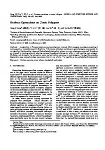
SPEED-UP OF EVM-BASED BOOLEAN OPERATIONS JORGE RODRIGUEZ*, DOLORS AYALA** *CEMVICC - Universidad de Carabobo **LSI - Universidad Politecnica de Catalu˜na (
[email protected],
[email protected])
Abstract Manipulation of volume representations is nowadays a very challenger goal in the field of scientific visualization. Boolean operations are an important tool to achieve edition tasks over volumetric representations such as merging between objects, detection of overlapping and cutting of pieces. Thus, acceleration techniques to speed-up boolean operations are an important goal in order to provide edition operations with response times near to interactivity. This paper presents a new approach to achieve EVM-based boolean operation faster than the conventional way.
1 Introduction In recent papers, the Extreme Vertices Model (EVM) has been reported as a competitive representation scheme to visualize and manipulate volume data, so an intermediate model between the voxelization and the final visualization has been defined using the EVM. A surface extraction technique based on the EVM allows to generate block-form isosurfaces without redundancy of primitives, and a properly defined set of operations allows to edit and manipulate the EVM-represented volume data. Boolean operations are well-defined on the EVM and they are the basis of most of the edition operations, so the implementation of acceleration techniques for these operations are always welcomed. This work presents an improvement of EVM-based Boolean operations using strategies based on bounding regions. Two different approaches were studied and implemented in order to improve the performance of the EVM-based Boolean operations. Considerable reductions in processing time haven been achieved when the overlapping between the operands is partial.
2
The Extreme Vertices Model
The Extreme Vertices Model (EVM) is a very concise representation scheme in which any orthogonal polyhedrom or pseudo-polyhedron (OPP) can be described using only a subset of its vertices: the extreme vertices. The EVM is actually a complete (nonambiguous) solid model: it is an implicit boundary representation (B-Rep) model, i. e., all the geometry and topological relations concerning faces, edges and vertices of the represented OPP can be obtained from the EVM. In the following we review the main definitions and properties to formally define the EVM. All concepts are more extensively explained and proved in previous work [AA98] and [Agu98].
2.1
Definitions
Let P be an orthogonal pseudo-polyhedron (OPP): • axis-prefixable: A linear element is axisprefixable when it is parallel to a prefixed axis. A planar element is axis-prefixable when it is perpendicular to the prefixed axis. • ABC-sorted: Let Q be a finite set of points in E 3 . We define the ABC-sorted set of Q as the set resulting from sorting Q according to coordinate A, then to coordinate B, and then to coordinate C. Thus, six possible ABC-sorted sets can be defined XYZ, XZY, YXZ, YZX, ZXY, and ZYX. • A brink or extended-edge is the maximal uninterrupted segment built out of a sequence of collinear and contiguous two-manifold edges of P . Moreover, an extended-face is the maximal set of coplanar and contigous faces, joined by lower dimensional elements (vertices or edges) of P . Brinks and extended-faces are axisprefixable.
• Extreme vertices (EV ) are the ending vertices of all brinks in P . EV (P ) ⊆ V (P ). V (P ) being the set of all vertices of P .
Y
X
• Extreme Vertices Model (EVM) of P is an ABCsorted set of all the extreme vertices of P . Any OPP is described by its (an only its) set of EV .
Z
A
• A plane of vertices (pov) of P is the set of vertices lying on a plane perpendicular to a main axis of P (usually the A axis). We will also refer as line of vertices (lov) to the set of brinks lying on a line parallel to a coordinate axis (usually the C axis). Planes and lines of vertices are axis-prefixable and we will refer to both of them as plv. • A slice is the region between two consecutive planes (or lines) of vertices. P can be expressed as the union of all its slicesSin a certain orthogonal direction. Hence, P = np−1 slicek (P ). k • A section (S) is the resulting polygon (or set of polygons) from the intersection between a slice of P and an orthogonal plane (or line) perpendicular to a certain orthogonal direction. . Sk (P ) will refer to the K th section of P between plvk (P ) and plvk+1 (P ). A slice from a 2D-OPP is a set of one or more disjoint rectangles, while a slice from a 3D-OPP is a set of one or more disjoint prisms, whose base is the slice’s section. Each slice has its representing section. Furtehrmore, it will be called external or internal section of P , respectively, if this intersection is empty or not. All these definitions can be extended to any dimension [BMP99]. In this work we are concerned with dimension ≤ 3. Figure 1(b) shows an OPP with a brink from vertex A to vertex E (both extreme vertices). In this brink, vertices B, C and D are nonextreme vertices. At the same figure, the planes of vertices (in dark grey) and sections (in light grey) perpendicular to the X axis are depicted.
2.2
Properties of the EVM
Let P be an OPP with n planes of vertices. S0 (P ) = Sn (P ) = ∅ Property 1: The coordinate values of non-extreme vertices can be obtained from EV coordinates.
B
C
D
E
a) S0 = φ
S1 Plv1
S2 Plv2
S3 Plv3
S4 Plv4
S6 = φ
S5 Plv5
Plv6
Figure 1. (a) An OPP P. (b) X-perpendicular planes of vertices and sections of P. (c) X-perpendicular faces of P: FD in black (pointing to the right) and BD in light grey (pointing to the left)
Property 2: Sections can be computed from planes of vertices and vice-versa. Si (P ) = Si−1 (P ) ⊗∗ plvi (P )
(1)
plvi (P ) = Si−1 (P ) ⊗∗ Si (P )
(2)
where plvi (P ) and Si (P ) denote the projections of plvi (P ) and Si (P ) onto a main plane parallel to P and ⊗∗ denotes the regularized XOR operation. Note that in order to operate with the projections we need not take into account the coordinate of the extreme vertices that corresponds to the projecting plane. Property 3: The computing of any plane of vertices can be decomposed into two terms that we will call forward difference and backward difference (FD and BD for short): For i = 1 . . . n
plvi (P ) = (Si−1 (P )−∗ Si (P ))∪(Si (P )−∗ Si−1 (P )) (3) and, thus, we can decompose it as:
F Di (P ) = (Si−1 (P ) −∗ Si (P )) ∗
BDi (P ) = (Si (P ) − Si−1 (P ))
(4) (5)
Property 4: F Di (P ) is the set of faces on plvi (P ) whose normal vector points to one side of the main axis perpendicular to plvi (P ), while BDi (P ) is the set of faces whose normal vector points to the opposite side. Figure 1(c) shows an OPP with its faces correctly oriented through FD and BD operations. Property 5: Let P and Q be two d-D (d ≤ 3) OPP, having EV M (P ) and EV M (Q) as their respective models, then, EV M (P ⊗∗ Q) = EV M (P ) ⊗ EV M (Q) (6)
Properties 3 y 4 provide proof that the EVM is a complete B-Rep model. Property 5 means that the XOR operation works in 0-D, because it is applied to the EV of the model. Therefore, sections are obtained from planes of vertices and vice-versa by applying the XOR operation to the extreme vertices.
3 The EVM-based Boolean operations In this section the EVM-Boolean operations algorithm is briefly depicted, a more detailed explanation can be found in [AA99] and [Agu98]. The algorithm basically performs a geometric merge between the orthogonal objects represented as a sorted EVM. The algorithms computes a sequence of 2D sections from the 3D model and the same algorithm is recursively applied to each of these 2D sections to obtain 1D sections (a list of collinear brinks). Then 1D Boolean operations are performed on these 1D sections. The recursion upwards by converting the resulting sequence of sections into an EVM, thus produces the corresponding result. Figure 2 illustrates the working of the algorithm. Literal (f) shows the merging between 2D sections for an union operation, generating the new 2D section of the resulting object.
4
Speed-up of EVM-based Booelan operations
From the explanation about of how the EVM-based Boolean operations work, it is obvious that only the overlapping region is relevant to obtain the correct result. The remaining planes of vertices are not modified, so they can be directly appended, if it would be the case, to the resulting object. Taking profit of this
Y X Z
b a
d
c
e
f
g
h
Figure 2. Boolean operations: 3D example. (a),(b) Two objects. (c),(d) Sections of the objects. (e) Objects in overlapping position. (f) Merging sections (union). (g) Computing new planes of vertices. (f)resulting object.
fact, strategies based on bounding regions can be implemented to accelerate the Boolean operations. The EVM-based Boolean operations are performed by traversing the scene in a fixed axisdirection (traversal direction). Thus, the overlapping region (critical region henceforth) will be computed according to that direction. The critical region will be defined as the region where the objects are overlapped with respect to the traversal direction. Therefore, the critical region is delimited by a pair of planes of vertices in the traversal direction. (see Figure 3). Once the critical region between two objects, A and B, has been computed, it can be empty or not. If it is empty, the objects are disjoints and the result of the operation is obvious. On the contrary, if the critical region is not empty, the domain of the operation is partitioned by two parallel planes, Π1 and Π2 , + − + into three half spaces: Π− 1 , (Π1 ∩ Π2 ), and Π2 . For simplicity, these three half spaces are notated as left, critical and right regions respectively: • Left region: Located at the negative region of Π1 , contains planes of vertices or brinks, belonging
A
Y
B
X Z
• Alef t , Bright : The left region is occupied by planes of vertices of EV M (A) and the right region is occupied by planes of vertices of EV M (B) exclusively • Aright , Blef t : The left region is occupied by planes of vertices of EV M (B) and the right region is occupied by planes of vertices of EV M (A) exclusively
Critical region
p1: y=u
p2: y=v
Figure 3. Critical region in Y-direction: the region contained between the planes y=u and y=v.
to A or B exclusively • Critical region: Located on the overlapping re− gion between Π+ 1 and Π2 zones, contains the planes of vertices or brinks of A and B involved in the operation.
• BinA: Left and right regions are occupied by planes of vertices of EV M (A) (the bounding region of B is completely contained by the bounding region of A) • AinB: Left and right regions are occupied by planes of vertices of EV M (B) (the bounding region of A is completely contained by the bounding region of B) At the figure 4(a) the case Alef t , Bright has occurred. For simplicity, a 2D representation is presented. Figure 4(b) shows remarked the planes of vertices inside the critical region.
• Right region: Located at the positive region of Π2 , contains planes of vertices or brinks, belonging to A or B exclusively. Based on this partitioning of the domain, two different approach of partitioning of the EVM can be defined: • Partitioning the EVM based on planes of vertices • Partitioning the EVM based on brinks In the critical region, a conventional Boolean operation is performed upon the one-dimensional sections (chain of brinks), but the treatment varies according to the previous approaches. Both of them have been analyzed and implemented in this work, and they are described in the following sections.
4.1 Approach 1: Based on planes of vertices In this first approach, the planes of vertices of EVMrepresented objects involved in the operation are divided among the three regions. Let A and B be two non-disjoint EVM-represented objects, the following casuistic is produced:
Figure 4. Partitioning based on planes of vertices
In the critical region, a conventional Boolean operation is performed between such pieces (A∗ and B ∗ )
of the original objects which lies inside it. Computing the operation between A∗ and B ∗ , requires that both pieces are considered as two objects. It can be achieved using the sections to compute the planes of vertices on the limits of the critical region. At the Figure 4(a) the first plane of vertices of A∗ has to be computed, so the previous section to this point is required, but computing this one requires to determine the previous one and so on. This is true in general, so the computation of all sections previous to the critical region is required in this approach. For each partitioning configuration of the Plvs, and depending on the operation to be computed, the planes of vertices in the three regions are appended to the resulting EV M according to the assignation rules on the table 1. In short, the acceleration technique of the EVMbased Boolean operations based on the partitioning of the planes of vertices can be outlined as follows: 1.- Compute the bounding regions of A and B 2.- Compute the critical region 3.- Classify the planes of vertices in P lvsright , P lvslef t and P lvscritical 4.- Append planes of vertices to the resulting EVM following the assignation rules It is important to note that the algorithm processes the objects in a sorted way, so the planes of vertices can be read directly from the original EVMrepresented objects. Also, the resulting EVM is constructed already sorted. Therefore, no new collectors of Plvs have to be created and no additional sorting operations are required. Furthermore, the sorted traversal of the objects allows a progressive computation of the sections required to determine the first plane of vertices inside the critical region.
in this approach the objects are reduced to a mess of brinks, so they cannot be read directly from the EVMrepresented objects and new collectors of brinks have to be created. Therefore, in the classifying step, special care has to be taken to separate, in different sets, the brinks of the object A of the such ones belonging to the object B, generating six different sets of brinks: BrinksAright , BrinksAlef t , BrinksBright , BrinksBlef t , BrinksAcritical and BrinksBcritical . Actually, depending on the configuration of the regions, two of the first four sets are always empty. For example, in the Figure 5, BrinksAright and BrinksAlef t are empty.
Figure 5. Partitioning based on brinks
4.2 Approach 2: Based on brinks The second approach proposed to improve the EVMbased Boolean operations is based on the partitioning of the brinks, instead of the planes of vertices. In this case, the EVM of the objects is sorted in such way that the brinks are perpendicular to the planes of the critical region (parallel to the traversal direction). Then, all the brinks are classified with respect to the three regions and such of them which begin in a region and finish in another one are split. A similar casuistic to the previous case is generated, but in terms of brinks instead of planes of vertices. See Figure 5. However,
Once all the brinks have been split (if it would be the case) and classified, the pieces of the objects inside the critical region (A∗ and B ∗ ) are actually welldefined EVM-represented objects. Therefore, this approach has the advantage that the computation of successive sections previous to the critical region is unnecessary. However, some additional ordering operations are required to convert the messes of brinks into valid EVM-represented objects. Furthermore, a postprocess to unify the split brinks has to be performed. All these shortcomings are avoided in the previous ap-
case 1: Aright , Blef t P lvsright P lvslef t P lvscritical case 2: Alef t , Bright P lvsright P lvslef t P lvscritical case 3: B ⊂ A P lvsright P lvslef t P lvscritical case 4: A ⊂ B P lvsright P lvslef t P lvscritical
union all all ∗ A ∪ B∗
difference (A-B) all ∗ A − B∗
intersection ∗ A ∩ B∗
all all A∗ ∪ B ∗
all A∗ − B ∗
A∗ ∩ B ∗
all all ∗ A ∪ B∗
all all ∗ A − B∗
∗ A ∩ B∗
all all A∗ ∪ B ∗
A∗ − B ∗
A∗ ∩ B ∗
Table 1. Plvs assignation rules.
proach by processing the objects in the traversal direction, which has not any sense in this approach. In this approach, the brinks assignation rules are defined on the table 2. BrinksAright BrinksBright BrinksAlef tt BrinksBlef t Brinkscritical
union all all all all A∗ ∪ B ∗
difference all all A∗ − B ∗
intersection A∗ ∩ B ∗
celerate EVM-based Boolean operations. The testing operand objects are the skull dataset (96 × 96 × 69) and a translated version of itself (see figure 6). All the algorithms have been run on a Sun Ultra Sparc 60 workstation. The processing time for each Boolean operation is presented on the table 3.
Table 2. Brinks assignation rules. Two of the first four sets are always empty.
The algorithm for this approach can be outlined as follows: 1.- Compute the bounding regions of A and B 2.- Compute the critical region 3.- Classify the brinks (splitting when it is necessary) 4.- Append, to the resulting EVM, all the brinks according to the assignation rules 5.- Unify split brinks and sort the resulting EVM.
5 Experimental Results The results presented in this section correspond to the implementation of both previous approaches to ac-
Figure 6. testing operands. Although the approach 2 (App. 2) avoids to compute the sections previous to the critical region, the required sorting operations introduce delay in the performance. Therefore, in general, the approach 1 has better performance. An exception occurs in the intersection case because this operation discards the sets of brinks outside of the critical region, so the ordering of these brinks and the brinks unifying process
Union Intersection Difference
Conventional 9.87 4.69 7.36
App. 1 6.57 2.14 4.95
App. 2 8.6 1.87 5.86
Table 3. Acceleration techniques processing time (in seconds)
are saved. A detailed inspection of processing time of the sub-processes for the intersection operation, confirms this hypothesis. Approach 1:
Boolean operations, the method based on planes of vertices has proved to be better at the most of times. Unfortunately, the acceleration achieved is strongly related to the intersection configuration between the bounding boxes of the operands. On the future, an integrated model for surface and direct volume rendering is going to be defined using the EVM. These accelerated Boolean operations will be integrated to this integrated model in order to provide edition capabilities over the EVM-represented volume data.
References [AA98]
A. Aguilera and D. Ayala. Domain extension for the extreme vertices model (EVM) and set-membership classification. In CSG’98. Ammerdown (UK), pages 33 – 47. Information Geometers Ltd., 1998.
[AA99]
D. Ayala and A. Aguilera. The extreme vertices model (evm) for orthogonal polyhedra. Geometric Modeling. DagstuhlSeminar-Report; 240, 1999.
• Proc. time of the Plvs at the left region: 0.38s. • Proc. time of the Plvs inside the critical region: 1.25s. • Proc. time of the Plvs at the right region: 0.33s. • Proc. time of closing the final EVM: 0.18s Approach 2: • Proc. time of classifying of brinks: 0.47 s. • Proc. time of intersection inside the critical region: 1.27s. • Proc. time of appending outside brinks: 0s. • Proc. time of re-unifying the split brinks: 0s. • Proc. time of re-ordering final set of brinks: 0.13s. In the detailed information it is possible to see that the time reported for the approach 2 for the steps 3 and 4 is null, because no more brinks have to be added to the resulting set, and no re-unifying of brinks is required.
6
Conclusions and future work
We have presented two different strategies to speedup the computing of Boolean operations using EVMrepresented objects. Both proposed approaches are based on bounding regions techniques, but the partitioning scheme along the regions is quite different. Although both strategies speed-up the performance with respect to the conventional implementation of
[Agu98] A. Aguilera. Orthogonal Polyhedra: Study and Application. PhD thesis, LSIUniversitat Polit`ecnica de Catalunya, 1998. [BMP99] O. Bournez, O. Maler, and A. Pnueli. Orthogonal Polyhedra: Representation and Computation. In Hybrid Systems: Computation and Control, LNCS 1569, pages 46 – 60. Springer, 1999.