Department of Computer Science, University of Illinois at Urbana- ... {jtchang,
dmedwrds, yyz}@uiuc.edu ..... ACM Computing Surveys, 27(3):433–467, 1995.
Statistical Estimation of Fluid Flow Fields Johnny Chang
David Edwards
Yizhou Yu
Department of Computer Science, University of Illinois at Urbana-Champaign Urbana, IL 61801, USA {jtchang, dmedwrds, yyz}@uiuc.edu
Abstract
Since we would like to focus on the motion analysis of fluids, we need to consider the features present in fluid dynamics. A fluid whose density and temperature are nearly constant is described by a velocity field u and a pressure field p. These quantities generally vary both in space and in time and depend on the boundaries surrounding the fluid. Given that the velocity and the pressure are known for some initial time t = 0, the evolution of these quantities over time follows the Navier-Stokes equations [5, 9]:
Many natural phenomena involve dynamic fluids whose motion differs radically from that of rigid bodies. This paper presents a novel approach for estimating fluid motion fields. It first estimates a local flow probability distribution function at each pixel using the STAR model and the data from a spatio-temporal neighborhood. It then feeds the set of distribution functions into a global optimization framework. As a result, the optimization returns a motion field with a unique velocity vector at each pixel. Experiments with real fluid sequences show that this method can successfully estimate their motion fields.
du dt
= =
∇·u =
1 Introduction
∂u + (u · ∇)u ∂t 1 − ∇p + ν∇2 u + f ρ 0
(3) (4)
where ν is the kinematic viscosity of the fluid, ρ is its density and f is an external force. The velocity field here can be either two-dimensional or three-dimensional. The first equation bears a resemblance to Eq.(2) except that its unknown variable is the velocity vector itself and the righthand side of the equation is not likely to be zero because of external forces such as gravity, the gradient field of pressure and diffusion. The second equation means the fluid is incompressible and volume-preserving. Based on the motion of fluids described by the NavierStokes equations, we understand that fluids have nonrigid motion. That means relative positions among points in a fluid change constantly at every possible scale. A good example is the changing surface geometry of a water surface. This is because the self-advection term (u·∇)u can quickly distort the relative positions of neighboring points to invalidate the assumption that neighboring points share the same flow vector. Other terms in the Navier-Stokes equations, such as diffusion, make this problem even more severe. For instance, the diffusion of smoke particles in the air changes the distribution of participating media, adding another level of nonrigidity. In summary, fluid motion is the opposite of rigid body motion. As a result, traditional optical flow methods based on affine neighborhood matching would have a difficult time estimating the projected motion
Dynamic fluids, such as rivers, ocean waves, moving clouds, smoke and fires, appear everywhere in the nature. They give us visual richness as well as spiritual inspiration. Nonetheless, they may also interfere with vision tasks such as image registration and geometry reconstruction. Good understanding and estimation of their motion can lead to more universal and robust vision algorithms. On the other hand, fluid motion estimation can also be very useful in synthesizing dynamic textures [16, 14, 15]. Optical flow is the traditional method to estimate motion fields. The initial hypothesis in optical flow methods is that the intensity structures of local time-varying image regions are approximately constant under motion for at least a short duration. Formally, if I(x, t) is the image intensity function, then I(x, t) ≈ I(x + δx, t + δt). (1) Expanding the right-hand side and ignoring second and higher order terms, we have the optical flow constraint equation, ∂I dI = + ∇I · v = 0 (2) dt ∂t Since the above equation has two unknowns, usually we assume all the pixels in a local block share the same flow vector to overconstrain the problem. 1
field of a 3D fluid in an image. Meanwhile, in time series analysis, there are some models that have shown potential to model the behavior of fluids. The autoregressive(AR) model has been often used for predicting the value of a state variable s at time t. The forecast is a linear combination of some number, m, of previous values: st = A1 st−1 + · · · + Am st−m + nt
are ignorable. In this paper, we are interested in natural gray-scale or color images where pixel intensities are not related to volumetric fluid properties and distortions due to projection may be significant. Therefore, we will not explicitly make use of these physical properties. In terms of temporal texture modeling, Szummer and Picard [16] applied the STAR model to analyze and resynthesize homogeneous temporal textures. Soatto et.al. [15] adopted PCA and AR model fitting to the analysis and synthesis of temporal textures and achieved broader and better results. Sch¨odl et.al. [14] addresses the same problem by finding transition points in the original video sequence where the video can be looped back on itself. A global image registration approach for scenes with temporal textures is presented by Fitzgibbon [6].
(5)
where the At are r × r(s ∈ Rr ) matrix constants which characterize the sequence. The term n t is drawn from a zero-mean noise distribution, typically taken to be Gaussian. This AR model can be generalized to include a spatial neighborhood as well. The result is the spatio-temporal autoregressive model (STAR) which does prediction using a linear combination of the values in a spatio-temporal neighborhood: s(x, y, t) =
m �
2 Local Flow Probability Distribution Functions
Ai s(x+∆xi , y +∆yi , t+∆ti )+n(x, y, t)
In this paper, we still assume that the brightness of a point is a constant over a short period of time. However, a statistical approach for determining flow vectors should be adopted instead since the relative positions of neighboring points change faster in a fluid than on a rigid body. Based on the characteristics of fluid motion, we can build a stochastic fluid motion model. The flow vector at a pixel at a certain time can be considered as a random variable with a probability distribution function. This probability distribution function at a pixel (x s , ys ) at a certain time t can be represented as, φxs ,ys ,t (xd , yd ), (xd , yd ) ∈ Ds , where D s is the set of destination pixels � ( which is often a neighborhood of pixel (xs , ys ) ) and (xd ,yd )∈Ds φxs ,ys ,t (xd , yd ) = 1. We assume that pixels in a local spatio-temporal region centered at (xs , ys , t) share the same probability distribution function for their flow vectors. The flow vector at each pixel in the local spatio-temporal region can be considered as a random sample from this distribution function. Therefore, the statistics of the flow vectors in the local region can be used as an approximation to this distribution function. Once we have the estimation of the probability distribution function, the flow vector at the center pixel (x s , ys ) is more likely to be consistent with a vector with a high probability. For the reasons mentioned in Section 1, recovering probability distribution functions for flow vectors becomes more achievable than recovering accurate pixelwise flow vectors for each frame. The STAR model appears to be very useful for estimating local distribution functions. Let us first look at Eq. (6) more carefully. The coefficient A i indicates the degree of correlation between pixel (x, y) at time t and pixel (x + ∆xi , y + ∆yi ) at time t + ∆ti . When a causal neighborhood is assumed, intuitively, A i is proportional to the probability of the fluid at pixel (x + ∆x i , y + ∆yi ) actually ending up at pixel (x, y) after a time interval −∆t i . How-
i=1
(6) where ∆xi , ∆yi and ∆ti specify the neighborhood structure of the model. The STAR model only exploits first and second-order statistics, hence cannot model curved lines.
1.1 Related Work There is a large body of literature on optical flow algorithms which can be roughly grouped into differential, correlation and frequency-based approaches. More specifically, there are a few representative frameworks, including the iterative first-order approximation method by Lucas and Kanade [11], the hierarchical computational framework [1, 4], the phase-based approach by Fleet and Jepson [7], the spatiotemporal filtering framework [8, 17], the mixture framework for motion segmentation [19] etc. Beauchemin and Barron [2] gives an excellent survey on this problem. Some of the above approaches have been adapted to estimate fluid flows. Quenot et.al. [13] presented an optical flow technique based on the use of dynamic programming along the two orthogonal major axes. It also incorporates neighborhood matching. Artificial particles are deposited into the fluid to provide more salient features in the images. The computed flow fields from real images are roughly consistent with numerical simulations. Larsen et. al. [10] adapted the phase-based approach to estimating flow fields in meteorological images. Some other work explicitly incorporates the physical properties of fluid mechanics during flow estimation, such as the use of the conservation of brightness or mass in [20, 3], the coupling between dense and parametric vector fields in [12]. This approach works well for meteorological and transmittance images where either 3D fluid properties are preserved or distortions caused by 3D to 2D projection 2
ever, if we consider pixel (x, y) as the source of flow instead of destination and assume ∆t i > 0 for all i, the STAR model still has legitimate physical interpretation where A i is proportional to the probability of the event that the fluid at pixel (x + ∆xi , y + ∆yi ) actually comes from pixel (x, y). To estimate the probability distribution function at pixel (xs , ys ), we need to have an estimation of the probability that the fluid at pixel (xs , ys ) goes to pixel (xs + ∆xi , ys + ∆yi ) at the next frame, which means ∆t i = 1, for all i. In Eq. (6), s(x, y, t) can be either state variables or appearance variables. Since we keep the brightness constancy assumption, s(x, y, t) can actually be replaced by image pixel intensity. Taking the expectation of the both sides of Eq. (6) and setting ∆ti = 1, we have I(x, y, t) =
m �
Ai I(x + ∆xi , y + ∆yi , t + 1)
fitting. This is not a severe problem since D s is twodimensional and N s is three-dimensional in general. However, pruning can definitely further improve the results. For flow distribution functions, pruning means setting some of their insignificant coefficients to zero. To efficiently carry out pruning, we actually use the Schwartz’s Bayesian Criterion (SBC) [18] and a binary search to decide the number of nonzero coefficients. Insignificant coefficients can be discarded as long as the SBC decreases. The expression of SBC is given by SBC = |Ω| ln σ ˆa2 + p ln |Ω|,
where |Ω| is the data set size, p is the number of coefficients, and σ ˆa2 is the estimated innovation variance. The binary search performs as follows. Given the initially estimated coefficients and their corresponding SBC value (sbc0 ), set half of the coefficients with smallest magnitude to zero and execute least-squares again for the remaining coefficients to obtain a new SBC value, sbc 1 . Comparing the two resulting values of SBC, we can decide which half of the coefficients we need to further work on. If sbc0 > sbc1 , the set of nonzero coefficients may still be redundent and recursively execute the previous step on this set; otherwise, restore the original values of the zero coefficients and recursively execute the previous step on them. This binary search can efficiently recover the necessary number of nonzero coefficients in the flow distributin function and reduce the amount of uncertainty in them.
(7)
i=1
where Ai becomes exactly the probability that the intensity at pixel (x + ∆xi , y + ∆yi ) in the next frame equals the intensity at pixel (x, y) in the current frame. Therefore, φxs ,ys ,t (xs + ∆xi , ys + ∆yi ) ≈ Ai
(8)
where (xs + ∆xi , ys + ∆yi ) ∈ D s . Since what we need to estimate is a distribution function with multiple parameters, the amount of data available from a single pixel (xs , ys ) is obviously not sufficient. As mentioned previously, the same distribution function is used for describing the statistical behaviour of all pixels in a spatiotemporal neighborhood N s of (xs , ys , t), which means we can have an equation similar to Eq. (7) for every pixel in N s . This is a linear equation in the set of distribution coefficients and we assume a Gaussian noise source at every pixel. The distribution coefficients can be solved using the system of normal equations for least-squares when the number of pixels in N s is larger than the number of pixels in Ds . Compared with [16] which adopts the STAR model for synthesizing homogeneous temporal textures, our work tries to use it for local flow distribution functions which vary from place to place. Although the STAR model is linear and inappropriate for global curved flow structures, it can still effectively model all local flows very well since even curved flow structures have a first-order local approximation. � The least-squares estimation does not guarantee that i Ai = 1 which is a necessary condition for a distribution function. Thus, Eq. (8) should be adapted to Ai φxs ,ys ,t (xs + ∆xi , ys + ∆yi ) ≈ � j Aj
(10)
3 Global Optimization The previous section introduced a method to recover local flow probability distribution functions. A local distribution function defines the probability of every potential velocity vector at a pixel. However, the motion field of a dynamic fluid actually has a unique velocity vector everywhere. In this section, we present an optimization-based method to extract a dense motion field with a unique velocity vector everywhere from the set of local distribution functions. The underlying idea for this two-stage approach is that the pixelwise velocity vectors should be determined simultaneously in a global framework which exploits the local information from all pixels. A local probability distribution function has this kind of required information available. A local approach could determine the velocity vector at every pixel only from its own distribution function. For instance, it could just pick the vector with the largest probability from each distribution function separately. The upcoming sections are going to be focused on the global optimization. Our global method formulates the problem as an unconstrained minimization problem with a cost function. It follows the Bayesian framework to maximize a posterior distribution for the global motion field.
(9)
2.1 Pruning Since fluid motion is largely random and noisy, the flow distribution function needs to be overdetermined during data 3
h(0, 0) = 1; ii) h(x, y) = 0, |x| ≥ 1 or |y| ≥ 1; iii) hx (0, 0) = 0 and hy (0, 0) = 0; iii) hx (x, y) = 0 if |x| = 1 or |y| = 1, and hy (x, y) = 0 if |x| = 1 or |y| = 1. Obviously, Eq. (12) and Eq. (13) become equivalent when (∆xs , ∆ys ) happens to be an integer vector.
The posterior distribution is obtained from a prior distribution and an observation model.
3.1 Cost Related to Smoothness One of the most important features of a fluid flow field is that it should be smooth. Smoothness is enforced on the flow field as a prior distribution in the Bayesian framework. If the spatial derivatives of the global flow field {u} are implemented using the following finite differences: ux (xs , ys ) = u(xs + 1, ys ) − u(xs , ys ) and uy (xs , ys ) = u(xs , ys + 1) − u(xs , ys ), then the prior distribution of the flow field may be described by a Gibbs distribution p({u}) = (1/Zprior ) exp(−λU ), where Zprior is a normalization constant and the energy term is given by � � �ux (xs , ys )�2 + �uy (xs , ys )�2 . (11) U= s
3.3 The Complete Cost Function The final posterior distribution for a global flow field can be formulated as being proportional to � (14) φ˜xs ,ys ,t (xs + ∆xs , ys + ∆ys ) exp(−λU ) s
Maximizing the above posterior distribution is equivalent to minimizing the following cost function. � ˜ − s log(φxs ,ys ,t (xs + ∆xs , ys + ∆ys )) � (15) + λ s (�ux (xs , ys )�2 + �uy (xs , ys )�2 )
s
The above complete cost function may have many local minima especially because of the first term. Usually expensive simulated annealing is adopted to optimize such a cost function. We designed an alternative heuristic optimization procedure which couples the fast conjugate gradient algorithm with a changing support region for the basis function h(x, y). The conjugate gradient algorithm is executed on the cost function multiple times. Every time, it takes the final solution from the previous step as the initial solution in the current step. Set to a value larger than the size of D s at the beginning, the support region for the basis function is shrunk by a fixed scaling factor every step until it reaches 1. In practice, we find out this scheme works well and always finds a vector field close to the optimal solution.
This probability distribution assigns high probability to fields that exhibit small derivatives and low probability to fields with high spatial derivatives.
3.2 Cost Related to Probability Distribution Functions Note that the observations we have made here are not the original input image sequence, but the set of local flow probability distribution functions derived from the images. The observation model relates the set of observed local distribution functions to any particular realization of the global flow field. It models the joint conditional probability of the observed distribution functions given the actual realization of the underlying global flow field, and can be expressed as � φxs ,ys ,t (xs + ∆xs , ys + ∆ys ) P ({φ}|{u}) = (1/Zobs )
4 Experimental Results
s
We have conducted experiments on multiple fluid sequences and compared the results from our algorithm with those obtained from two of the previous optical flow algorithms, including Lucas and Kanade’s multi-scale algorithm [11] and an improved version of Quenot et.al.’s algorithm [13] whose original version works very well for fluids with artificial particles. Their results are shown side-by-side with our results in the Figs. 1-3. Most previous optical flow algorithms estimate flow fields using only two consecutive frames while ours estimates the local flow distribution functions from multiple frames, so direct comparison between them is not entirely appropriate. Nevertheless, it does indicate that our algorithm provides a working technique for dynamic fluids. The test image sequences themselves provide strong visual cues about the flow directions, therefore, we can evaluate the correctness of the results.
(12) where Zobs is a normalization constant, u(x s , ys ) = (∆xs , ∆ys ) defines a flow vector at pixel (x s , ys ), and should be maximized over. Usually a differentiable cost function is required for gradient-based optimization techniques. But the flow probability distribution functions recovered in the previous section are only discrete functions defined over integer vectors (∆xi , ∆yi ). To convert Eq. (12) into a differentiable function, we decide to apply a locally supported basis function, h(x, y), at each integer vector location. Thus, P ({φ}|{u}) in Eq. (12) becomes � (1/Z˜obs ) s φ˜xs ,ys ,t (xs + ∆xs , ys + ∆ys ) � � = (1/Z˜obs ) s { i [φxs ,ys ,t (xs + ∆xi , ys + ∆yi ) h(∆xs − ∆xi , ∆ys − ∆yi )]} (13) where (xs + ∆xi , ys + ∆yi ) ∈ Ds , and h(x, y) is a differentiable function satisfying the following conditions: i)
Smoke Sequence: The first experiment illustrates the results on a smoke sequence. Two consecutive images from 4
(a)
(c)
(e)
(b) (a)
(b)
(c)
(d)
(e)
(f)
(d)
(f)
Figure 1. (a)-(b) Two consecutive frames from a smoke sequence; (c) flow field from Lucas and Kanade’s algorithm; (d) flow field from Quenot et.al.’s algorithm; (e) flow field from our algorithm without global optimization; (f) flow field from our algorithm with global optimization;
Figure 2. (a)-(b) Two consecutive frames from a spiraling water sequence; (c) flow field from Lucas and Kanade’s algorithm; (d) flow field from Quenot et.al.’s algorithm; (e) flow field from our algorithm without global optimization; (f) flow field from our algorithm with global optimization;
the sequence are shown in Fig. 1(a)-(b). They indicate there is a wind from left to right. The estimated flow fields for the bottom part of the images are shown in Fig. 1(c)-(f). Fig. 1(c) shows the results from Lucas and Kanade’s algorithm. Fig. 1d shows the results from Quenot et.al.’s algorithm. Fig. 1(e) shows our results without global optimization by choosing the locally optimal vectors from the flow distribution functions. Fig. 1(f) shows our results with global optimization. The recovered flow fields from our approach agree well with visual observation.
estimation. The estimated flow fields are shown in Fig. 2(c)-(f). Our algorithm does not perform as well on this sequence partially due to the low quality of the images. But it still produces reasonable results with the correct swirling direction. Ocean Wave Sequence: The third sequence that has been tried is the ocean wave sequence with a huge tidal wave falling from the top. We can also approximately tell the flow directions from the images in Fig. 3(a)-(b). The estimated flow fields are shown in Fig. 3(c)-(f). Our algorithm performed very well on this sequence.
Spiraling Water Sequence: The second experiment was perfomed on the spiraling water sequence originally from [16]. The counterclockwise flow directions are visually noticeable in the example images shown in Fig. 2(a)(b). Compared with smoke, water sequences have more sparkling highlights that interfere more severely with flow
From the above results, we can see that overall our algorithm performs much better than Lucas and Kanade’s and Quenot et.al.’s. The version with global optimization also 5
References
(a)
(b)
(c)
(d)
(e)
(f)
[1] P. Anandan. A computational framework and an algorithm for the measurement of visual motion. International Journal of Computer Vision, 2:283–310, 1989. [2] S.S. Beauchemin and J.L. Barron. The computation of optical flow. ACM Computing Surveys, 27(3):433–467, 1995. [3] D. Bereziat, I. Herlin, and L. Younes. A generalized optical flow constraint and its physical interpretation. In Proc. of CVPR, 2000. [4] J.R. Bergen, P. Anandan, K.J. Hanna, and R. Hingorani. Hierarchical model-based motion estimation. In Proc. ECCV, pages 237–252, 1992. [5] A.J. Chorin and J.E. Marsden. A Mathematical Introduction to Fluid Mechanics. Springer-Verlag, New York, 1990. Texts in Applied Mathematics 4. [6] A.W. Fitzgibbon. Stochastic rigidity: Image registration for nowhere-static scenes. In Proc. Intl. Conf. Computer Vision, 2001. [7] D.J. Fleet and A.D. Jepson. Computation of component image velocity from local phase information. Int. J Comput. Vision, 5(1):77–104, 1990. [8] D.J. Heeger. Optical flow using spatiotemporal filters. Int. J Comput. Vision, 1:279–302, 1988. [9] L.D. Landau and E.M. Lifshitz. Fluid Mechanics. Butterworth-Heinemann, Oxford, 1998. [10] R. Larsen, K. Conradsen, and B.K. Ersboll. Estimation of dense image flow fields in fluids. IEEE Trans. Geoscience and Remote Sensing, 36(1):256–264, 1998. [11] B.D. Lucas and T. Kanade. An iterative image registration technique with an application to stereo vision. In Proc. 7th Intl. Joint Conf. on Art. Intell., 1981. [12] E. Memin and P. Perez. Fluid motion recovery by coupling dense and parametric vector fields. In Proc. ICCV, 1999. [13] G.M. Quenot, J. Pakleza, and T.A. Kowalewski. Particle image velocimetry with optical flow. Experiments in Fluids, 25:177–189, 1998. [14] A. Schodl, R. Szeliski, D.H. Salesin, and I. Essa. Video textures. In Proceedings of Siggraph, pages 489–498, 2000. [15] S. Soatto, G. Doretto, and Y. Wu. Dynamic textures. In Proc. Intl. Conf. Computer Vision, pages 439–446, 2001. [16] M. Szummer and R.W. Picard. Temporal texture modeling. In Proc. ICIP, 1996. [17] J. Weber and J. Malik. Robust computation of optical flow in a multi-scale differential framework. International Journal of Computer Vision, 7:5–19, 1994. [18] W.W.S. Wei. Time Series Analysis: Univariate and Multivariate Methods. Addison-Wesley, 1995. [19] Y. Weiss and E.H. Adelson. A unified mixture framework for motion segmentation: incorporating spatial coherence and estimating the number of models. In Proc. of CVPR, 1996. [20] R. Wildes and M. Amabile. Physically based fluid flow recovery from image sequences. In IEEE CVPR, pages 969– 975, 1997.
Figure 3. (a)-(b) Two consecutive frames from an ocean wave sequence; (c) flow field from Lucas and Kanade’s algorithm; (d) flow field from Quenot et.al.’s algorithm; (e) flow field from our algorithm without global optimization; (f) flow field from our algorithm with global optimization;
performs better than the one with local decision by effectively suppressing noisy vectors. In all of the above experiments, we use a 11 by 11 spatial neighborhood for the set of destination pixels D s used in flow distribtion functions, and a 17x17x8 spatio-temporal neighborhhod N s for the leastsquares estimation of the coefficients in those flow distribution functions. The basis function h(x, y) was set to a tensor product of cosine functions, 0.25(cos πx + 1)(cos πy + 1). The parameter λ was set to a number larger than 10 to enforce smoothness.
Acknowledgments This work was supported by National Science Foundation CAREER Award CCR-0132970. We would like to thank the anonymous reviewers for their valuable comments. 6