American Journal of Mathematics and Statistics 2014, 4(4): 195-203 DOI: 10.5923/j.ajms.20140404.04
Statistical Project of X Control Chart with Variable Sample Size and Interval R. C. Leoni1, N. A. S. Sampaio2, R. C. M. Tavora2, J. W. J. Silva2,3,*, R. B. Ribeiro3 1
Universidade Estadual Paulista, UNESP, Guaratinguetá, SP, Brazil Associação Educacional Dom Bosco, AEDB, Resende, RJ, Brazil 3 Faculdades Integradas Teresa D’Ávila, FATEA, Lorena, SP, Brazil 2
Abstract Control charts with adaptive schemes are tools used to monitor processes and to signal the presence of special
causes. However, the use of adaptive schemes is not common yet because they are topics rarely covered in textbooks and are not available in traditional software used for statistical analysis. This work aims to present how to plan and estimate the optimal parameters of an adaptive chart for monitoring the mean of a process using sample size and variable interval ((X_bar-VSSI). The X_bar-VSSI chart was chosen because it is a scheme with great potential for practical application, for the chart only requires knowledge of the sample size and the time between sample selections after established the optimal parameters for the chart. Markov chains were used to evaluate the chart performance based on the average time between the instant when the process changes and the moment when the chart signals the condition out of control. It is presented two functions written in R language to assist the user in planning a statistical project based on the X_bar-VSSI adaptive scheme.
Keywords Statistical process control, Adaptive charts, Markov chains, R language
1. Introduction Control charts are used to monitor the production process in order to signal deviations from the target value of a quality characteristic that one wants to monitor. Detection of small or moderate deviations by traditional charts proposed by Shewhart [1] is slow, that is why several charts have been proposed. Some authors introduced the adaptive control charts which are called this way because they do not present all their fixed parameters. Construction of this kind of chart provides that at least one of its parameters may vary and it can be: the control limits, the sample size and the time interval in which a sample is collected. For instance, consider the chart of adaptive control in which vary the sample size and the time interval in which a sample is collected. In this scheme, according to information obtained by the most recent sample, one can modify the size and collect interval of next sample. Designing a control chart to use in practice, involves elaboration of a sampling plan by means of specification of sample size and time interval between removal of samples, and calculation of control limits. The mechanism which involves determination of limits distance of chart control at centerline is closely related to statistical testing of hypothesis. Extending the control limits decreases the risk of monitored * Corresponding author:
[email protected] (J. W. J. Silva) Published online at http://journal.sapub.org/ajms Copyright © 2014 Scientific & Academic Publishing. All Rights Reserved
statistics to be located beyond the control limits, with the adjusted process (error type I). However, extending the boundaries increases the risk of monitored statistic being located within the control limits when the process is out of adjustment, known as error type II [2]. In adaptive control charts, it is common to use Markov chains to evaluate the performance of chart according to the set of chosen parameters [3, 4, 5]. In order to assess the statistical properties, it is used the subjacent idea of dividing the variation interval of monitored statistic on a finite set of status. The transient statuses of the chain are located in the control region of chart and the absorbing status in the region established as out of control. The adaptive charts are not available in traditional statistical softwares, despite showing better performance than the charts with fixed parameters. Determination of adaptive parameters is not a trivial task, therefore, this paper proposes the use of a free software to plan and estimate the optimal parameters of an adaptive chart for X with
variable sample size and interval ( X − VSSI ). The average number of samples until the moment in which the chart indicates the out of control condition (ARL) and the average time between the instant at which the process is changed and the time when the chart indicates the out of control condition (ATS) are performance measures used as reference to parameters choice. The X − VSSI chart was chosen because it is a scheme with great potential for practical application, for the chart requires only knowledge of sample size and the time among samples selection after established the optimal parameters.
196
R. C. Leoni et al.: Statistical Project of
X
Control Chart with Variable Sample Size and Interval
The statistical properties of control chart are optimized considering the approach presented by Zimmer [4], ie, a Markov chain is used to establish the parameters keeping statistical risks type I and type II under control. The rest of the paper is organized as follows: section 2 presents the c control chart. In section 3, it is described the procedure to evaluate the performance of a X − VSSI chart using Markov chains.
2. The X − VSSI Control Chart
w < Zi −1 < k − w < Zi −1 < w (1) −k < Zi −1 < − w
Figure 1. The
the ith sample ( n(i ) = n1 < n(i ) =n2 ) ; h(i ) is the time
performed
to
remove
ith
the
sample
( h(i) =h1 > h(i) =h2 ) ; k and w are limits that define
control regions; Z i is control statistics calculated by:
( xi − µ0 ) . (σ 0 /
Z= i
n (i )
)
−1
(2)
Where xi is the sample mean of the ith subgroup;
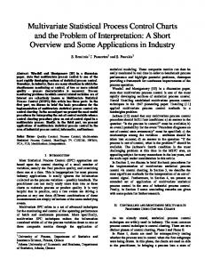
Reynolds [6] was the first to consider the adaptive design of control chart by varying the time interval in which a sample is collected. Then there appeared a large number of papers for the purpose of varying the other control chart parameters, being proven that this technique generally increases the chart power in detection of special causes just modifying the quality characteristic average (variable) that is desired to monitor [7-10]. The X − VSSI control chart is adaptive with respect to the sample size and time interval at which a sample is collected. This chart was used by Prabhu [11, 12], Costa [3] and Park [9] to monitor a process statistics. In a control chart with sample size and interval variables (see Figure 1), the sample size and the time interval in which a sample is collected can vary according to the information provided by the most recent sample collected. In this chart type, random samples of different sizes are collected at variable intervals of length according to the function:
( n2 , h1 ) if = ( n(i), h(i) ) ( n1, h2 ) if ( n , h ) if 2 1
where i = 1,2, ..., is the sample number; n(i ) is the size of
and
µ0
σ 0 are the mean and standard deviation of the process
when in control.
( n(i), t (i) ) depends on ( Zi −1 ) marked on the chart.
The choice between the pairs the position of the last point
For a chart X − VSSI , one can divide the control region in three mutually exclusive and exhaustive regions, as follows (see Figure 1): • Region within the alarm limits:
I1 =
[ − w, w] .
• Region between the limits for alarm and control:
I2 = •
I= 3
[ −k , − w ) ( w, k ] .
Region
outside
[ −∞, −k ) ( k , ∞ ] .
the
control
limits:
[ − w, w] , the control (or inspection) is relaxed using the pair ( n1 , h2 ) , If the statistic Z i falls within the region
I1 =
otherwise if the current point Z i lies within the region
[ −k , − w ) ( w, k ] , the control will be tighter by using the pair ( n2 , h1 ) . I2 =
X − VSSI control chart
American Journal of Mathematics and Statistics 2014, 4(4): 195-203
matrix obtained by:
3. The Performance of the X − VSSI Control Chart The statistical performance of a control chart can be evaluated by calculating the ARL and ATS statistics. Depending on the process operation conditions, one has the ARL when the process is in control (ARL0), that is, the expected number of samples between two successive false alarms and the ARL for process out of control (ARLδ), which represents the expected number of samples between the occurrence of special cause which alters the monitored parameter and signal triggered by the chart. Similarly, one has the ATS when the process is in control (ATS0), representing the average time between two successive false alarms and ATS for process out of control (ATSδ), representing the expected time between the occurrence of special cause and the signal triggered by the chart. It is possible to calculate the ARL and ATS statistics using Markov chains. One observes the expected number of transitions before the monitored statistic lies in the absorbing state of the chain. The Markov chain proposed in Zimmer [4] was used in this study to assess the ARL in control and out of control, ARL0 and ARLδ, respectively. Each transition probability is calculated as the probability of the statistic falls within one of the regions of the control range ( I1 , I 2 or I 3 ). In this chain, there are two transient states and one
absorbing state that corresponds to the process out of control. The state transition matrix of chain that represents the operation of process in control, P0 , can be divided into four
Φ ( w ) − Φ ( − w ) 2 Φ ( k ) − Φ ( w ) Q0 = (5) Φ ( w ) − Φ ( − w ) 2 Φ ( k ) − Φ ( w ) Where
Φ (.) denotes the standard normal cumulative
function; K and w are the limits that define the region of the chart control. The average time that the chart can produce a false alarm is:
= ATS0
R0 I
Q Pδ = δ 0
the absorbing state; 0 is the matrix that states the impossibility of going from an absorbing state to a transient state, and I is the identity matrix. In a Markov chain, the element (i, j) of the matrix
[ I − Q0 ]−1
represents the average number of visits to the j
transient state before reaching the absorbing state, given that the process started at the i state. Each control transition probability is calculated as the probability of a point of monitored statistic falls within one of the regions of the control range. Therefore, the average number of samples between two successive false alarms is calculated by:
= ARL0
T
−1
{b} [ I − Q0 ] {1}
(4)
{b}T is a vector with initial probabilities; I is the identity matrix; {1} is a unit vector and Q0 is a transition
where
Rδ I
(7)
= ARLδ
{b}T [ I − Qδ ]−1 {1}
(8)
= ATSδ
{b}T [ I − Qδ ]−1 {h}
(9)
And
being the transition matrix given by:
Qδ 12 Q Qδ = δ 11 Qδ 21 Qδ 22 where:
states; R0 is the transition matrix from transient states to
(6)
In order to calculate the performance measures ARLδ and ATSδ it is used:
(3)
Where Q0 is the transition matrix between transient
{b}T [ I − Q0 ]−1 {h}
where {h} is a vector with the sampling intervals. The transition matrix of the process running out of control is given by:
sub-matrices:
Q P0 = 0 0
197
( Qδ 21 = Φ ( w − δ
(10)
) ( ); n2 ) − Φ ( − w − δ n2 ) ;
Qδ 11 = Φ w − δ n1 − Φ − w − δ n1
(
) ( ) ( ) ( ) (
)
Qδ 12 = Φ k − δ n1 − Φ w − δ n1 + Φ −k − δ n1 − Φ − w − δ n1 Qδ 22 = Φ k − δ n2 − Φ w − δ n2 + Φ −k − δ n2 − Φ − w − δ n2
(
(
(
The vector with initial probabilities
)
{b}T
)
)
;
.
is defined
according to the initial conditions of operation in the process:
{b}T
Φ ( w ) − Φ ( − w ) 2 Φ ( k ) − Φ ( w ) = (11) Φ ( k ) − Φ ( −k ) Φ ( k ) − Φ ( −k )
R. C. Leoni et al.: Statistical Project of
198
X
Control Chart with Variable Sample Size and Interval
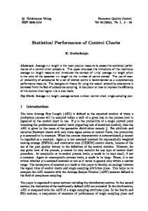
In this paper, it is considered the condition known as Steady-State, ie, it is assumed that the process starts in control and at some future instant, it occurs a special issue that causes a shift at the target value of monitored statistic. Planning a control chart can be formalized as an optimization problem in which the decision variables are the parameters of the chart. Figure 2 illustrates the objective function and constraints that define the best set of parameters of the X − VSSI chart.
Objective Function:
h1 =
n2 rinsp
(13)
where rinsp is the amount of parts (a piece, a component, etc.) which can be inspected per unit of considered time E (h) = h0 . For example, if rinsp = 60 given that
h0 = 1 hour, it is assumed that it is possible to inspect 60
min ATS ( n1, n2 , h1, h2 , w, k δ )
Subject to:
parts every hour. For more details, see Celano [13, 14]. Once defined h0, h1, w and k, h2 is obtained by means of the expected time to collect a sample:
E (n) = n0 ;
E (h= ) h= 0
ATS ( n1, n2 , h1, h2 , w, k δ= 0= ) ATS0 ;
E (h) = h0 ;
The optimization problem is finally reduced to finding the pair ( n1 , n2 ) which minimizes the objective function. The
nmin ≤ n1 ≤ n2 ≤ h1.rinsp Objective function and constraints for the parameters of the
X − VSSI
control chart
In Figure 2, n1 and n2 are the sample sizes; h1 and
h2 are the time intervals between samples collection; w
and k are control limits of the chart; δ is the displacement degree of occurred in the average of the process; ATS0 is
the mean time between two successive false alarms; n0 is
the expected value of the collected sample size with the process in control; h0 is the expected time to collect a sample with the process in control and
rinsp is the
quantity of parts (a piece, a component, etc.) which can be inspected per time unit considered in h0 .
In order to illustrate that the optimization problem is reduced to find the pair (n1,n2) that minimizes the objective function, consider without generality loss that E (h= ) h= 0 1 the time unit (for example: 1 hour, 0.5 hour
and etc.) and ARL0 = 370.4. Thus, AT S0 = ARL0 = 370.4 and k = 3. The expected value of the sample size with the process in control, E ( n) = n0 , is given by:
E (n= ) n= 0
2 Φ ( k ) − Φ ( w ) Φ ( w) − Φ ( −w) h1 + h2 Φ ( k ) − Φ ( −k ) Φ ( k ) − Φ ( −k ) (14)
0 < w < k; hmin ≤ h1 ≤ h2 ≤ hmax ; Figure 2.
expression (12). The shortest range of optimal sampling ( h1 ) is given by:
2 Φ ( k ) − Φ ( w ) Φ ( w) − Φ ( −w) n1 + n2 Φ ( k ) − Φ ( −k ) Φ ( k ) − Φ ( −k ) (12)
A pair of samples ( n1 , n2 ) is selected; since ( n1 , n2 ), n0 and k are known, w can be inferred directly from the
next section presents an application example of how to plan an optimal statistical project that shows which values for the pair ( n1 , n2 ) should be used. For this, it has been used the R software [15] to obtain the optimal parameters of a X − VSSI chart.
4. Example In this section, it is proposed two functions (see Appendix) developed for use in R environment that evaluate the performance of the X − VSSI control chart and solve the optimization problem shown in Figure 2. The R is a free software that allows the user to add functionality, making it flexible to generate statistical analyzes and receive contributions of many researchers through specific packages which are freely available in a central repository called CRAN (Comprehensive R Archive Network). The R can be obtained directly on the Internet at: http://www.r-project.org. The first function, called VSSI, evaluates the performance of the control chart calculating the ATSδ when supplied by the user: n1, n2, n0,delta ( δ ), h0 andr_insp. The second function, VSSI.optimum, solves the optimization problem shown in Figure 2. Here it is necessary to provide: n0,delta ( δ ), h0,r_insp and a value for nmax which is referred to the largest size of admissible sample to collect. In order to illustrate the use of functions, consider the example presented in Costa [16]. A packaging line has an average value of milk 1000 ml and standard deviation estimated to be 4.32 ml. Monitoring is performed in the process average by inspecting samples of size n0 = 5 at each time unit. Suppose that this unit is equal to h0=1 hour. In this example, the parameters planned for the control chart are
American Journal of Mathematics and Statistics 2014, 4(4): 195-203
fixed, ie, the sample size, the sampling interval and limits do not change after estimated. To use the X − VSSI control chart in the example shown it is necessary to calculate the control limits (w and k) and the sampling scheme and
( n2 , h1 )
. Choosing
( n1, h2 )
= n2 8 ) , keeping ( n1 2;=
n0 = 5 ; δ = 1, 0 ; ARL0 = 370.3983; ho = 1 hour (60 min.)
and r_insp = 60, the VSSI function provides the parameters shown in Figure 3. In this example, δ = 1.0 means that the process average went from µ0 = 1000 (in control) to µ= 1 µ0 + δ .σ 0
= 1000 + 1* 4.32 = 1004.32 (out of control). Consider the case in which δ = 2.0 . Figure 4 illustrates
the results obtained with the VSSI function. It is observed that the ATS is lower (ATSδ=2