Statistical Properties of Digital Piecewise Linear Chaotic ... - CiteSeerX

Statistical Properties of Digital Piecewise Linear Chaotic Maps and Their Roles in Cryptography and Pseudo-Random Coding? Li Shujun1a , Li Qi2 , Li Wenmin3 , Mou Xuanqin1b , and Cai Yuanlong1c 1

Institute of Image Processing, School of Electronics and Information Engineering, Xi’an Jiaotong University, Xi’an, Shaanxi 710049, P. R. China 2 Department of Electrical Engineering and Electronics, The University of Liverpool, Brownlow Hill, Liverpool L69 3GJ, UK 3 Department of Electircal and Electronic Engeering, Imperial College, Exhibition Road, London SW7 2BT, UK

Abstract. The applications of digital chaotic maps in discrete-time chaotic cryptography and pseudo-random coding are widely studied recently. However, the statistical properties of digital chaotic maps are rather different from the continuous ones, which impedes the theoretical analyses of the digital chaotic ciphers and pseudo-random coding. This paper detailedly investigates the statistical properties of a class of digital piecewise linear chaotic map (PLCM), and rigorously proves some useful results. Based on the proved results, we further discuss some notable problems in chaotic cryptography and pseudo-random coding employing digital PLCM-s. Since the analytic methods proposed in this paper can essentially extended to a large number of PLCM-s, they will be valuable for the research on the performance of such maps in chaotic cryptography and pseudo-random coding.

1

Introduction

Chaotic systems have many interesting properties, such as the sensitive dependence on initial conditions and control parameters, ergodicity, mixing and exactness properties, etc. [1]. Most properties can be connected with some requirements in cryptography and pseudo-random coding [2–4]. From 1990s, more and more researchers devote their contributions to a new field – chaotic cryptography; many analog and digital chaotic encryption systems have been proposed [2, 3, 5–9] and analysed [10–12]. As a general method to design chaotic stream ciphers, chaotic pseudo-random coding techniques are commonly used to construct PRBG-s (Pseudo-Random Bits Generators) [5,6,9]. At the same time, ?

This paper was published in Cryptography and Coding C Proceedings of the 8th IMA International Conference (IMA-C&C2001, December 17-19, 2001, Cirencester, UK), Lecture Notes in Computer Science, vol. 2260, pp. 205-221, Springer-Verlag, Berlin, 2001. Shujun Li is the corresponding author, personal web site: http://www.hooklee.com.

2

Li Shujun et al.

chaotic pseudo-random coding techniques have also developed separately in other areas, such as electronics, communications [13–15] and computer physics [16]. As we know, piecewise linear chaotic maps (PLCM) are the simplest kind of chaotic maps from the viewpoint of realization. What’s more, they have uniform invariant density and good correlation functions [17], which is very useful for cryptography and pseudo-random coding [18]. In fact, many researchers have used them to realize chaotic ciphers and PRBG-s [6–9, 14]. It seems that chaotic systems are perfect as a new rich source of cryptography and pseudo-random coding. Unfortunately, when chaotic systems are realized in finite computing precision, their digital dynamical properties will be far different from the continuous ones. Some severe problems will arise, such as short cycle length, non-ideal distribution and correlation functions, etc. Assume the finite precision is L (bits) and fixed-point arithmetic is adopted, it is the following reasons to cause such degradation: 1) All values represented with finite precision are binary rational decimals formulated as a/2L (a = 0 ∼ 2L −1). Since the Lebesgue measure of all the decimals is zero, they cannot represent the right dynamical behaviors of the chaotic systems defined on a real interval with positive measure; 2) There are only 2L digital values to represent the chaotic orbits, so the cycle length of the orbits will not be larger than 2L , generally it will be much smaller than 2L ; 3) The quantization errors, which are introduced into the iterations of chaotic systems, will make the chaotic orbits depart from the theoretical ones with uncontrolled manners (it is impossible to know the exact errors). Some researchers have noticed the degradation of digital chaotic systems [9–11, 13, 19, 20], and several remedies have been suggested: using higher finite precision [11,19], the perturbation-based algorithm [9,20], and cascading multiple chaotic systems [13]. Because it is difficult to measure the statistical properties of digital chaotic maps theoretically, experiments are generally used as the analytic tools to estimate the performance of the above remedies. However, sometimes experiments are not enough to tell us the right things about digital chaotic systems. The theoretical tools for digital chaotic systems are needed.

2

Outline of Our Works

In this paper, we strictly prove some interesting statistical properties about a class of digital PLCM with finite computing precision. Based on our proved results, we can explain some statistical degradation of digital PLCM-s theoretically. Such degradation will cause the chaotic ciphers insecure, and cause chaotic pseudo-random sequences unbalanced. Furthermore, we discuss the performance of the three proposed remedies, and point out none of them can essentially improve such degradation. But the perturbation-based algorithm is still useful in practice, since it can be carefully used to enhance the performance of digital chaotic ciphers and pseudo-random coding. For other digital chaotic maps, we have not yet obtained exact corresponding results. But our proof techniques may probably be extended to many other digital chaotic maps conceptually. If one chaotic map contains a control parameter that

Roles of PLCM in Cryptography & Pseudo-Random Coding

3

is proportional to uniformly distributed final output, the digital chaotic map may be weak from the viewpoint of this control parameter. In the future, we will try to find more delicate results. This paper is organised as follows. In Sect. 3, we firstly introduce some preliminary knowledge. In the following Sect. 4, we focus on the mathematically rigorous proofs of the interesting properties of digital PLCM-s. Since the whole proof is rather lengthy, it is divided into several parts. Based on the proved properties, we explain what they mean in chaotic cryptography and pseudo-random coding in Sect. 5. A brief conclusion is given in the last section.

3 3.1

Preliminary Knowledge Piecewise Linear Chaotic Map (PLCM)

Generally, given a real interval X = [α, β] ⊂ R, a piecewise linear chaotic map F : X → X is a multi-segmental map: i = 1 ∼S m, F (x)|Ci = Fi (x) = ai x + bi , where m {Ci }m is a partition of X, which satisfies i=1 i=1 Ci = X and Ci ∩ Cj = ∅, ∀i 6= j. Each element of the partition is mapped to X by Fi : ∀i = 1 ∼ m, Fi : Ci → X. Such a map has the following statistical properties on its definition interval X : 1) it is chaotic, its Lyapunov exponent λ satisfies 0 < λ < ln m; 2) it is exact, mixing and ergodic, and has uniform invariant density function f (x) = 1/(β−α); 1 PN −1 (x − x ¯)(xi+n − x ¯) will go to zero 3) the correlation τ (n) = 12 lim N i i=0 σ N →∞ as n → ∞, where x ¯, σ are the mean value and the variance of x respectively; especially, if some conditions are satisfied, τ (n) = δ(n) [1, 17]. As we know [1], the uniform invariant density function means that uniform input will generate uniform output, and that the chaotic orbit from almost every initial condition will lead to the same uniform distribution f (x) = 1/(β − α). But such a fact is not true for a digital chaotic map, this paper will point out that uniform digital input cannot generate uniform digital output for all control parameters. Such a fact will subsequently cause serious dynamical degradation when the maps are iterated again and again. Because it is inconvenient to analyse chaotic maps with uncertain formulas, in this paper, we focus our attention on the following specific PLCM used in [8]:  x/p, x ∈ [0, p)  F (x, p) = (x − p)/(1/2 − p), x ∈ [p, 1/2] , (1)  F (1 − x, p), x ∈ [1/2, 1] where p is the control parameter, which satisfies 0 < p < 1/2. In order to facilitate the descriptions and proofs of the statistical properties in Sect. 4, we give some definitions in Sect. 3.2 and related results in Sect. 3.3. 3.2

Preliminary Definitions

 Pn Definition 1. A discrete set Sn = a a = i=1 ai · 2−i , ai ∈ {0, 1} is called a digital set with resolution n; ∀i < j, Si is called the digital subset with

4

Li Shujun et al.

resolution i of Sj . Specially, define S0 = {0}, S∞ = [0, 1), then we have {0} = S0 ⊂ S1 ⊂ . . . ⊂ Si ⊂ . . . ⊂ S∞ = [0, 1). Definition 2. Define Vi = Si −Si−1 (i ≥ 1) and V0 = S0 . Vi (0 ≤ i ≤ n) is called the digital layer with resolution i; ∀p ∈ Vi , i is called the resolution of p. The partition of Sn , {Vi }ni=0 , is called the complete multi-resolution decomposition of Sn ; {Vi }∞ i=0 is called the complete multi-resolution decomposition of S = [0, 1). For Sn , its resolution n is also called decomposition level, ∞ Sn i=0 Vi = Sn , and ∀i 6= j, Vi ∩ Vj = ∅. Definition 3. ∀n > m, Dn,m = Sn − Sm is called the digital difference set of the two digital sets with parameters n and m. {Vi }ni=m = {Si − Si−1 }ni=m is called the complete multi-resolution decomposition of Dn,m , n − m + 1 is called the decomposition level. Definition 4. A function G : R → Z is called an approximate transformation function (ATF), if ∀x ∈ R, |G(x) − x| < 1. Three basic ATF-s are: 1) bxc – the maximal integer not greater than x; 2) dxe – the minimal integer not less than x; 3) round(x) – the rounded integer of x. ∀x ∈ R, define its decimal part x − bxc as function dec(x). The above three ATF-s have the following useful properties (please note not all ATF-s): ATF Property 1 : ∀m ∈ Z, G(x + m) = G(x) + m; ATF Property 2 : a < x < b ⇒ bxc ≤ G(x) ≤ dxe.

(2) (3)

The proofs of the two properties are rather simple, we omit them here. Definition 5. A function Gn : S∞ → Sn is called a digital approximate transformation function (DATF) with resolution n, if ∀x ∈ S∞ = [0, 1), |Gn (x)−x| < 1/2n . The following three DATF-s are concerned in this paper (they are also the most frequently adopted DATF-s in digital computing algorithms): 1) floorn (x) = bx · 2n c/2n ; 2) ceiln (x) = dx · 2n e/2n ; 3) roundn (x) = round(x · 2n )/2n .4 The above three DATF-s have the following useful properties (please note not all DATF-s): DATF Property 1 : ∀m ∈ Z, Gn (x + m/2n ) = Gn (x) + m/2n ; DATF Property 2 : a < x < b ⇒ floorn (a) ≤ Gn (x) ≤ ceiln (b).

(4) (5)

The two properties are easily derived from the ATF Property 1–2. 3.3

Preliminary Lemmas about the Three Basic ATF-s

For the three basic ATF-s – b·c, d·e and round(·), we have two fundamental lemmas and one corollary, which will be useful in the proofs of the theorems in the next section. 4

Consider 1 ∈ / S∞ , without loss of generality, define ceiln (x) = 0 if dx · 2n e = 2n , and define roundn (x) = 0 if round(x · 2n ) = 2n . Such redefinitions will not essentially influence the following results since dec(1) = 0.

Roles of PLCM in Cryptography & Pseudo-Random Coding

5

Lemma 1. ∀n ∈ Z+ , a ≥ 0, the following three facts are true: 1. n · bac ≤ hbn · ac ≤ n · bac + (n − 1), and n · bac = bn · ac when and only when 1 ; dec(a) ∈ 0, n 2. n · dae − (n − 1) ≤ dn dae, and n · dae − (n − 1) = dn · ae when and  · ae ≤ n· S 1,1 only when dec(a) ∈ 1 − n {0}; 3. n · round(a) − bn/2c ≤ round(n · a) ≤ n · round(a) + bn/2c, and h  S hn · round(a) − 1 1 bn/2c = round(n · a) when and only when dec(a) ∈ 0, 2n 1 − 2n , 1 . The proof of this lemma is given in Appendix A. Corollary 1. ∀n ∈ Z+ , a ≥ 0, we have the following results: h  1 ; 1. bn · ac ≡ 0 (mod n) when and only when dec(a) ∈ 0, n   1 , 1 S{0}; 2. dn · ae ≡ 0 (mod n) when and only when dec(a) ∈ 1 − n  h  h 1 S 1 − 1 ,1 . 3. round(n·a) ≡ 0 (mod n) when and only when dec(a) ∈ 0, 2n 2n Proof. This corollary can be derived directly from the above lemma. 0 + 0 Lemma 2. ∀j,N, N odd integers satisfying 2j |(N + N 0 ),  0∈ Zj  , and N, N0 are j j we have N/2 + N /2 = (N + N )/2 − 1.

The proof of this lemma is given in Appendix B.

4

Statistical Properties of Digital PLCM

Give a one-dimensional chaotic map F (x, p) : I → I, where I = S∞ = [0, 1). When the finite precision is n, its digital version can be expressed by Fn (x, p) = Gn ◦ F (x, p) : Sn → Sn , where Gn (·) is a DATF, floorn (·), ceiln (·) or roundn (·). Denote the corresponding ATF of Gn (·) as G0 (·). Assume Pj denotes the probability of the lowest j bits of Fn (x, p) are all zeros, i.e., the probability of Fn (x, p) belongs to Sn−j : Pj = P {Fn (x, p) ∈ Sn−j }. For the map denoted by (1)5 , ∀p ∈ Vi ⊂ Si ⊆ Sn (2 ≤ i ≤ n), we can deduce some interesting results about Pj (1 ≤ j ≤ n), which are rather different from the expected ones based on the perfect continuous statistical properties of the map. Moreover, the results can be essentially extended to all digital PLCM-s described in Sect. 3.1. Because the whole proof is rather lengthy, we divide it into several parts: firstly a fundamental lemma, then the results about Pj (i ≤ j ≤ n) and the ones about Pj (1 ≤ j < i), finally two comprehensive theorems. 5

Because 1 ∈ / S∞ , redefine Fn (1/2, p) = 0. Consider F 2 (1/2, p) = 0 and dec(1) = 0, such redefinition will not essentially influence the following results.

6

4.1

Li Shujun et al.

A Fundamental Lemma

Firstly, we introduce Lemma 3, which gives some useful results about the highest n − i bits and the lowest i bits of Fn (x, p). This lemma is the fundamental of the following proofs. At the same time, this lemma reflects some facts about the local linearity of the PLCM-s, which makes the obtained results in this paper conceptually available for other PLCM-s. Lemma 3. ∀p ∈ Di,0 = Si − {0}(1 ≤ i ≤ n), x ∈ Sn . Assume p = Np /2i , x = Nx /2n , where Np , Nx are integers satisfying 1 ≤ Np ≤ 2i −1 and 0 ≤ Nx ≤ 2n −1. we have the following three results: 1. Gn (x/p) ∈ Sn−i ⇔ Nx ≡ 0 (mod Np ), bNx /Np c , 2. floorn−i (Gn (x/p)) = 2n−i 1 G0 (2i · (Nx mod Np )/Np ) 3. Gn (x/p) mod n−i = . 2n 2

(6) (7) (8)

N /N bNx /Np c + (Nx mod Np )/Np Nx /2n = xn−i p = , we Np /2i 2 2n−i G (2i · bNx /Np c + 2i · (Nx mod Np )/Np ) have Gn (x/p) = 0 . From ATF Property 2n 1, we can rewrite Gn (x/p) as follows Proof. Because x/p =

bNx /Np c G0 (2i · (Nx mod Np )/Np ) + . (9) 2n 2n−i Let us discuss the above equation under the following two conditions: bNx /Np c a) When Nx mod Np = 0: Gn (x/p) = + 0 ∈ Sn−i ; 2n−i b) When Nx mod Np = k 6= 0: Obviously 1 ≤ k ≤ Np − 1. Considering p < 1, we have 2i /Np > 1, then 1 < 2i · (Nx mod Np )/Np < 2i − 1. Thus, from ATF Property 2, 1 ≤ G0 (2i · (Nx mod Np )/Np ) ≤ 2i − 1. Therefore, Gn (x/p) =

bNx /Np c bNx /Np c 2i − 1 1 ≤ G (x, p) ≤ ⇒ Gn (x, p) ∈ / Sn−i . (10) + + n n 2 2n 2n−i 2n−i From a) and b), we can deduce Gn (x/p) ∈ Sn−i ⇔ Nx ≡ 0 (mod Np ). bNx /Np c At the same time, when Nx mod Np = 0, floorn−i (Gn (x/p)) = ; 2n−i   i bNx /Np c + 1/2 bNx /Np c when Nx mod Np = k 6= 0, floorn−i (Gn (x/p)) ≥ = 2n−i 2n−i   bNx /Np c + (2i − 1)/2i bNx /Np c and floorn−i (Gn (x/p)) ≤ = , so finally we 2n−i 2n−i bNx /Np c can get floorn−i (Gn (x/p)) = . 2n−i From the above result and (9), the following result is true: Gn (x/p) mod The proof is complete.

1 2n−i

=

G0 (2i · (Nx mod Np )/Np ) . 2n

Roles of PLCM in Cryptography & Pseudo-Random Coding

4.2

7

Results about Pj (i ≤ j ≤ n)

Theorem 1. Assume random variable x distributes uniformly in Sn , for the digital PLCM (1), ∀p ∈ Di,1 (2 ≤ i ≤ n)6 , we have: Pi = 4/2i . Proof. Assume p = Np /2i , x = Nx /2n , where Np , Nx are integers that satisfy 1 ≤ Np ≤ 2i − 1 and 0 ≤ Nx ≤ 2n − 1. Because x distributes uniformly in Sn , Nx will distribute uniformly in integer set [0, 2n − 1]. Since the chaotic map is defined piecewisely, we consider it on different segments: a) x ∈ [0, p) ⇒ Nx ∈ [0, 2n−i · Np − 1]: Fn (x, p) = Gn (x/p), from Lemma 3, we know Fn (x, p) ∈ Sn−i when and only when Nx ≡ 0 (mod Np ). Because Nx distributes uniformly in [0, 2n − 1], the probability of Fn (x, p) ∈ Sn−i will be 2n−i /(2n−i · Np ) = 1/Np . That is to say, Pi |x ∈ [0, p) = 1/Np . b) x ∈ [p, 1/2): Assume x0 = x − p, p0 = 1/2 − p, we have Fn (x, p) = x0 /p0 , where x0 ∈ [0, p0 ). Similarly to a), define p0 = Np0 /2i , x0 = Nx0 /2n , we will get Pi |x ∈ [p, 1/2) = Pi |x0 ∈ [0, p0 ) = 1/Np0 . c) x ∈ [1/2, 1): Consider the map is even symmetric to x = 1/2, we can easily get the following two results: Pi |x ∈ (1/2, 1 − p] = 1/Np0 and Pi |x ∈ ((1 − p, 1) ∪ {1/2}) = 1/Np . Here please note that 1 ∈ / Sn and 1/2 takes its position that is symmetrical to 0, which will not make any difference to Pi . From a) – c) and the total probability rule, we can deduce: Pi = P (x ∈ [0, p)) · Pi |x ∈ [0, p) + P (x ∈ [p, 1/2)) · Pi |x ∈ [p, 1/2) + P (x ∈ (1/2, 1 − p]) · Pi |x ∈ (1/2, 1 − p] + P (x ∈ ((1 − p, 1) ∪ {1/2})) · Pi |x ∈ ((1 − p, 1) ∪ {1/2}) 1 1 1 1 1 1 1 4 1 + p0 · 0 + p0 · 0 + p · = i+ i+ i+ i = i . =p· Np Np Np Np 2 2 2 2 2 The proof is complete. Theorem 2. Assume random variable x distributes uniformly in Sn , for the digital PLCM (1), ∀p ∈ Di,1 (2 ≤ i ≤ n), floorn−i (Fn (x, p))7 distributes uniformly in Sn−i . Proof. Similarly to the proof of Theorem 1, assume p = Np /2i , x = Nx /2n , we separately consider the map on different segments: a) x ∈ [0, p) ⇒ Nx ∈ [0, 2n−i · Np − 1]: Fn (x, p) = Gn (x/p), from Lemma 3, we have floorn−i (Fn (x, p)) = bNx /Np c/2n−i . Because x distributes uniformly in Sn , Nx distributes uniformly in [0, 2n−i · Np − 1]. Thus bNx /Np c distributes uniformly in [0, 2n−i − 1], i.e., floorn−i (Fn (x, p)) distributes uniformly in Sn−i when x ∈ [0, p). 6

7

Please note p should also satisfy 0 < p < 1/2 for the map (1). But such a fact will not essentially influence the theorems proved in this paper, we omit this requirement of p. This note is also available for the following theorems. The highest n − i bits of Fn (x, p).

8

Li Shujun et al.

b) x ∈ [p, 1/2): Assume x0 = x − p, p0 = 1/2 − p, we have Fn (x, p) = x0 /p0 , where x0 ∈ [0, p0 ). Similarly to a), we can prove floorn−i (Fn (x, p)) distributes uniformly in Sn−i when x ∈ [p, 1/2). c) x ∈ [1/2, 1): Because the map is even symmetrical to x = 1/2, it can be easily deduced that floorn−i (Fn (x, p)) distributes uniformly in Sn−i when x ∈ [1/2, 1). From a) – c), we know it is true that floorn−i (Fn (x, p)) distributes uniformly in Sn−i . The proof is complete. Theorem 3. Assume random variable x distributes uniformly in Sn , for the digital PLCM (1), ∀p ∈ Di,1 (2 ≤ i ≤ n) and i ≤ j ≤ n, Pj = 4/2j holds. Proof. Let us discuss the different conditions when j = i and j > i. a) j = i: From Theorem 1, Pj = 4/2i = 4/2j ; b) i < j ≤ n: Assume bm (m = 1 ∼ n) represents the mth bit (from the lowest  j−i  z }| { bit to the highest one) of Fn (x, p), Pj = P Fn (x, p) ∈ Sn−i ∧ bj · · · bi+1 = 0 · · · 0 .   Recall the proof of Theorem 2, when Fn (x, p) ∈ Sn−i (i.e., Nx mod Np = 0), bNx /Np c (the highest n − i bits of Fn (x, p)) still distributes uniformly in 1 = 4 · 1 = 4. [0, 2n−i − 1]. So we can get Pj = P {Fn (x, p) ∈ Si } · j−i 2 2i 2j−i 2j j From a) and b), we have: i ≤ j ≤ n ⇒ Pj = 4/2 . The proof is complete. 4.3

Results about Pj (1 ≤ j < i)

Firstly, we introduce Lemma 4 and Corollary 2, which will be used to facilitate the proof of Theorem 4. Lemma 4. Assume n is an odd integer, random integer variable K distributes uniformly in Zn = [0, n − 1], the following fact is true: K 0 = f (K) = (2i · K) mod n distributes uniformly in Zn , i.e., ∀k ∈ [0, n − 1], P {K 0 = k} = 1/n. Proof. As we know, (Zn , +) is a finite cyclic group of degree n, and a is its generator when and only when gcd(a, n) = 1, where “+” is defined as “(a + b) mod n” (see Theorem 2 on page 60 of [21]). Therefore, a = 2i mod n is one generator of Zn since gcd(a, n) = gcd(2i , n) = 1. Consider K 0 = (2i ·K) mod n = (a · K) mod n, we can see f : Zn → Zn is a bijection. Then we will immediately deduce: K 0 = f (K) distributes uniformly in Zn because K distributes uniformly in Zn . That is to say, ∀k ∈ [0, n − 1], P {K 0 = k} = 1/n. The proof is complete. Corollary 2. Assume n is an odd integer, random integer variable K distributes uniformly in Zn = [0, n − 1]. Then dec(2i · K/n) distributes uniformly in S = {x|x = k/n, k ∈ Zn }. Proof. This corollary is the straightforward result of the above lemma.

Roles of PLCM in Cryptography & Pseudo-Random Coding

9

Theorem 4. Assume random variable x distributes uniformly in Sn , for the digital PLCM (1), ∀p ∈ Vi (2 ≤ i ≤ n)8 and 1 ≤ j ≤ i − 1, we have:  1/2j + 2/2i , Gn (·) = floorn (·) or ceiln (·)  1/2j , 1 ≤ j ≤ i − 2 Pj = . , Gn (·) = roundn (·)  4/2i , j = i − 1 Proof. p = Np /2i , x = Nx /2n , where Np , Nx are integers that satisfy 1 ≤ Np ≤ 2i − 1 and 0 ≤ Nx ≤ 2n − 1. Because x distributes uniformly in Sn , Nx will distribute uniformly in integer set [0, 2n − 1]. Let us consider the digital map on different segments: a) x ∈ [0, p) ⇒ Nx ∈ [0, 2n−i ·Np −1]: Fn (x, p) = Gn (x/p), from Lemma 3, we know the lowest i bits of Fn (x, p) are determined by G0 (2i · (Nx mod Np )/Np ). Then we can deduce Fn (x, p) ∈ Sn−j ⇔ G0 (2i · (Nx mod Np )/Np ) ≡ 0 mod 2j . ˆ = Nx mod Np , which distributes uniformly in [0, Np − 1] because Define N ˆ )/Np , we can re-write of the uniform distribution of Nx . Define a = (2i−j · N i j G0 (2 · (Nx mod Np )/Np ) as G0 (2 · a). From Corollary 1, we can get:  h  , G0 (·) = b·c 0, 1j    2 S {0} , G0 (·) = d·e 1 − 1j , 1 . G0 (2j ·a) ≡ 0 (mod 2j ) ⇔ dec(a) ∈  2 Sh h    1 , 1 , G (·) = round(·)  0, 1 1 − j+1 0 2j+1 2 (11) From Corollary 2 (please note p ∈ Vi ensures Np is an odd integer), we know dec(a) = k/Np (k = 0 ∼ Np − 1)with uniform probability.

(12)

Based on (11) and (12), we can deduce:   Np   0, , G0 (·) = b·c    2j     S N k∈ Np − jp , Np {0} , G0 (·) = d·e .  2        Np S Np   Np − j+1 , Np , G0 (·) = round(·)  0, j+1 2 2

(13)

Consider k is an integer, we can get the probability  bNp /2j c + 1   , G0 (·) = b·c or d·e  Np P G0 (2j · a) ≡ 0 (mod 2j ) = . j+1   2 · bNp /2 c + 1 , G0 (·) = round(·) Np (14) 8

Please note the condition p ∈ Vi , NOT p ∈ Di,1 in Theorem 1–3.

10

Li Shujun et al.

b) x ∈ [p, 1/2): Assume x0 = x − p, p0 = 1/2 − p, we have Fn (x, p) = x0 /p0 , where x0 ∈ [0, p0 ). Similarly to a), define p0 = Np0 /2i , x0 = Nx0 /2n , we will get  bNp0 /2j c + 1   , G0 (·) = b·c or d·e   Np0 P G0 (2j · a0 ) ≡ 0 (mod 2j ) = , 0 j+1 2 · bNp /2 c + 1    , G (·) = round(·) 0 Np0 (15) ˆ 0 )/Np0 , N ˆ 0 = Nx0 mod Np0 . where a0 = (2i−j · N From (14) and (15), we can get the conditional probability Pj |x ∈ [0, 1/2). Consider the map is even symmetrical to x = 1/2, the final probability will be Pj = 2 · (Pj |x ∈ [0, 1/2)). In the following, we separately consider the condition of Gn (·) = floorn (·) or ceiln (·) and Gn (·) = roundn (·): i) Gn (·) = floorn (·) or ceiln (·), i.e., G0 (·) = b·c or d·e: p + p0 = 1/2 ⇒ Np + 0 Np = 2i−1 ⇒ 2j |(Np + Np0 ), from Lemma 2, we can deduce:   0 j bNp /2j c + 1 0 bNp /2 c + 1 + p · Pj =2 p · Np N0   p j 0 j i−j−1 bNp /2 c + bNp /2 c + 2 −1+2 = 1 + 2 . =2 =2 2i 2i−1 2j 2i

(16)

ii) Gn (·) = roundn (·), i.e., G0 (·) = round(·): When j < i − 1, Np + Np0 = 2 ⇒ 2j+1 |(Np + Np0 ), from Lemma 2, we can get: i−1

 0 j+1 c+1 2 · bNp /2j+1 c + 1 0 2 · bNp /2 Pj =2 p · +p · Np N0

  p j+1 0 j+1 2 bNp /2 c + bNp /2 c + 2 2 2i−j−2 − 1 + 2 =2 = = 1j . 2i 2i−1 2 

(17)

When j = i − 1, Np + Np0 = 2i−1 ⇒ 2j+1 - (Np + Np0 )(j + 1 = i > i − 1), Lemma 2 cannot be used, but we can calculate the probability Pj by directly observing (14) and (15): Np < 2i , Np0 < 2i , so Np /2j+1 < 1 ⇒ bNp /2j+1 c = 0, Np0 /2j+1 < 1 ⇒ bNp0 /2j+1 c = 0, then we have 

2·0+1 2·0+1 Pj = 2 p · + p0 · Np Np0

 =2·

2 4 = i. i 2 2

(18)

From (16) – (18),we can directly get the final result. The proof is complete. 4.4

Comprehensive Results about Pj (1 ≤ j ≤ n)

In the above subsections, we have separately proved the results about Pj (i ≤ j ≤ n) and Pj (1 ≤ j < i) for any p ∈ Vi ⊂ Si ⊆ Sn (2 ≤ i ≤ n). To make the above “rough-and-tumble” results tidier, we rearrange them into two new theorems, which are easier to be understood and to be used in practice.

Roles of PLCM in Cryptography & Pseudo-Random Coding 0

−1

−1

−2

−2

11

−3

log2Pj

log2Pj

−3

−4

−4

−5

−5 −6 −6 −7 −7 −8

−8

−9

−9

−10

1

2

3

4

5

6

7

8

j

(a) Gn (·) = floorn (·) or ceiln (·)

9

10

−10

1

2

3

4

5

6

7

8

9

10

j

(b) Gn (·) = roundn (·)

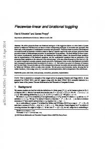
Fig. 1. Pj (1 ≤ j ≤ n) when p = 3/16 ∈ V4 ⊂ S4 , where the finite precision n = 10 (The line marked with diamond signs denotes the probability under digital uniform distribution 1/2j , and the other line denotes the probability Pj )

Theorem 5. Assume random variable x distributes uniformly in Sn , ∀p ∈ Vi (2 ≤ i ≤ n), the following results are true for the digital PLCM (1):   4/2j , i ≤ j ≤ n 1. When Gn (·) = roundn (·), Pj = 4/2i , j = i − 1 ;  1/2j , 1 ≤ j ≤ i − 2  4/2j , i≤j≤n 2. When Gn (·) = floorn (·) or ceiln (·), Pj = ; j 1/2 + 2/2i , 1 ≤ j ≤ i − 1  n−i n−i n−i 3. ∀k ∈ [0, 2 − 1], P floorn−i (Fn (x, p)) = k/2 = 1/2 . Proof. the first two parts are the combinations of Theorem 3 and 4, the last part is just equivalent to Theorem 2. Remark 1. If x distributes uniformly in the digital set Sn , Fn (x, p) does not distribute uniformly in Sn (but its highest n-i bits does in Sn−i , ∀p ∈ Si ), since Pj = 1/2j if Fn (x, p) distributes uniformly in Sn . To understand what Theorem 5 really means, see Fig. 1 for more visual details. Remark 2. Note there is an absolutely weak control parameter p = 1/4 ∈ V2 ⊂ S2 , which satisfies P2 = 4/22 = 1. That is to say, the lowest 2 bits of Fn (x, p) will always be zeros. In addition, ∀x0 ∈ Vi (2 ≤ i ≤ n), after at most di/2e iterations, the chaotic orbit will converge at zero: ∀m ≥ di/2e, F m (x0 ) = 0. Theorem 6. Assume random variable x distributes uniformly in Sn , and Pi = P {Fn (x, p) ∈ Sn−i }. The following results are true for the digital PLCM (1): Si 1. ∀p ∈ Di,1 = Si − S1 = k=2 Vi , Pi = 4/2i ; 2. ∀p ∈ Vi+1 , Pi = 4/2i+1 ;

12

Li Shujun et al. −3 −3.2 −3.4 −3.6

log2P5

−3.8 −4 −4.2 −4.4 −4.6 −4.8 −5 0

0.05

0.1

0.15

0.2

0.25

0.3

0.35

0.4

0.45

0.5

p

Fig. 2. P5 = P {Fn (x, p) ∈ Sn−5 } with respect to p, where n = 10, Gn (·) = floorn (·) (The dashed line denotes 2−5 , the ideal probability under digital uniform distribution)

 3. ∀p ∈ Vj (j ≥ i + 2), Pi =

1/2i , Gn (·) = roundn (·) . 1/2i + 2/2j , Gn (·) = floorn (·) or ceiln (·)

Proof. This theorem is an equivalent form of Theorem 5. Remark 3. Theorem 6 tells us: for the control parameters p with different resolution (i.e., in different digital layers of Dn,1 ), rather large difference exists in the generated chaotic orbits. Hence, from the observation of P1 ∼ Pn , one can get the resolution of the control parameter p. In Fig. 2, we give the experimental result of P5 with respect to p when n = 10 and Gn (·) = floorn (·), which entirely coincides with Theorem 6. 4.5

Extension to Other Digital PLCM-s

Although the above results are based on the specific PLCM denoted by (1), they can be essentially extended to all PLCM-s described in Sect. 3.1, of course the exact results will be different for different maps. From the proofs of theorems in above sub-sections, we can see that the statistical degradation occurs because of the piecewise linearity (Lemma 3 and 4) and the essential properties of the three ATF-s (Lemma 1 and 2). Employing Lemma 1–4 and Corollary 1–2 on other PLCM-s9 , we can easily obtain results corresponding to Theorem 5 and 6. For example, we can get the results about the following chaotic map:  x/p , x ∈ [0, p) F (x, p) = , (19) (1 − x)/(1 − p), x ∈ [p, 1] 9

Any PLCM defined on interval [α, β] can be re-scaled to its topologically conjugated PLCM defined on [0, 1] with a linear function h(x) = (x − α)/(β − α).

Roles of PLCM in Cryptography & Pseudo-Random Coding

13

where p satisfies 0 < p < 1. This map is one of the simplest PLCM-s, and generally called tent map. Theorem 50 . Assume random variable x distributes uniformly in Sn , ∀p ∈ Vi (1 ≤ i ≤ n), the following results are true for digital tent map:   2/2j , i ≤ j ≤ n 1. When Gn (·) = roundn (·), Pj = 2/2i , j = i − 1 ;  1/2j−1 , 1 ≤ j ≤ i − 2  2/2j , i≤j≤n 2. When Gn (·) = floorn (·) or ceiln (·), Pj = ; 1/2j + 1/2i , 1 ≤ j ≤ i − 1 3. ∀k ∈ [0, 2n−i − 1], P {floorn−i (Fn (x, p)) = k/2n−i } = 1/2n−i . Experiments show the results absolutely right. Of course there is the corresponding Theorem 60 , we omit it here since it is just another form of Theorem 50 .

5

The Roles of Digital PLCM-s in Cryptography and Pseudo-Random Coding

0

−1

−2

log2P5

−3

−4

−5

−6

−7

−8

0

0.05

0.1

0.15

0.2

0.25

0.3

0.35

0.4

0.45

0.5

p

Fig. 3. P50 = P {Fn32 (x, p) ∈ Sn−5 } with respect to p, where n = 10, Gn (·) = floorn (·) (P50 is the probability after 32 chaotic iterations of the digital PLCM (1), the dashed line denotes 2−5 , the ideal probability under digital uniform distribution)

From remark 1, we can know that a uniformly distributed digital signal will lead to non-uniform distribution after iterations of a digital PLCM. Such nonuniformity will become more and more severe as the iterations go, see Fig. 3 for some intuitional view (compare it with Fig. 2, the probability at most control parameters increases, and the probability at p = 1/16 even reaches to 1). We

14

Li Shujun et al.

can use the probability Pi to denote the degree of such non-uniformity: for a fixed control parameter, the larger Pi is, the larger the degradation will be. In remark 2, p = 1/4 ∈ V2 corresponds to the most serious degradation, so it is the weakest control parameter. The less weak control parameters are ones in V3 ; then those in V4 , V5 , · · ·. 5.1

Performance of the Three Remedies to Digital PLCM-s

In Sect. 1, we have mentioned three remedies proposed by other researchers. In this subsection, we discuss whether they will work well to improve the degradation of digital PLCM-s. Apparently, cascading multiple digital chaotic maps cannot essentially improve the weaknesses, since multiple cascading PLCM-s are just equivalent to a new PLCM with more segments. Using higher precision cannot change the weaknesses of any fixed control parameter either. For example, for the map (1), p = 1/4 will always be absolutely weak for any finite precision, and ∀p ∈ Vi will always be same weak for any finite precision n ≥ i. But higher precision will introduce more stronger digital layers10 and then improve the overall weakness, which makes the condition better. Now assume the perturbation-based algorithm is used to improve the degradation of digital PLCM-s. We find there exists a “strange” paradox: assume the chaotic orbit {x(m)}∞ m=1 is improved to obey nearly uniform by perturbation, according to Theorem 5 and 6, the chaotic sub-orbit {x(m)}∞ m=2 will not obey ∞ ∞ uniform distribution because {x(m)}∞ = {F (x(m), p)} n m=2 m=1 ; thus {x(m)}m=1 will not either. What does such a fact mean? It implies the non-uniformity revealed by the above theorems is the lower bound of the degradation of digital chaotic orbits. In other words, the perturbation-based algorithm cannot essentially improve the degradation to a better condition than the one depicted in Theorem 5 and 6. However, as we will point out in the next subsection, the perturbation-based algorithm is still useful to enhance the digital chaotic ciphers and pseudo-random coding with careful considerations. 5.2

Notes on Chaotic Ciphers and Pseudo-Random Coding

If the digital PLCM-s are directly used in chaotic ciphers and the control parameter are used as the secret key (as most chaotic ciphers do), the cryptographic properties of the ciphers will not be perfect, and many weak keys will arise (see Fig. 3), because of the severe degradation induced by the digital chaotic iterations. To escape from such a bad condition and enhance the security, we suggest using the perturbation-based algorithm as follows: the perturbation is secretly exerted and the chaotic orbit is output after perturbation (See Fig. 4). It is based on the following fact: if {x(m)}∞ m=1 can be observed by one intruder, he 10

When finite precision increases from n to n0 , n0 − n stronger digital layers Vn0 −n+1 ∼ Vn0 will be added, although n old digital layers V1 ∼ Vn remain.

Roles of PLCM in Cryptography & Pseudo-Random Coding

K1

K2

-

15

Perturbing PRNG

? A -

Digital Chaotic System

? B -L

Key-stream

Fig. 4. Digital chaotic cipher with secretly exerted perturbation (The perturbation should be secretly exerted at position B not A)

will probably judge the resolution i of the right key through the probabilities Pj (j = 1 ∼ n) (see Theorem 6 and Remark 3), and then search the key only in the digital layer Vi that is smaller than the whole key space (the smaller i is, the faster the search will be and the weaker the key). If the perturbation is exerted secretly at point B, one intruder can only observe perturbed {x(m)}∞ m=1 not {x(m)}∞ m=1 itself, then it is relatively more difficult for him to get information about K1 without knowing K2 . But it is obvious that K1 will still be weak if K2 is broken, and vice versa. It means the final key entropy will be smaller than the sum of the two sub ones: H(K) = H((K1 , K2 )) < H(K1 ) + H(K2 ). If the digital PLCM-s are used to generate pseudo-random bits, the generated binary sequences may be unbalanced since the chaotic orbits are not uniform. For example, if the map denoted by (1) with p = 1/4 is selected and the lowest 2 bits of chaotic orbit are used to generate pseudo-random bits, we can see they will be 000 · · ·. Fortunately, from Theorem 2, we can use the highest n-i bits to construct desired pseudo-random bits. Here please note (approximately) uniform distribution of chaotic input is required. The perturbation-based algorithm will be useful for such a task.

6

Conclusion

We have rigorously proved some statistical properties of digital piecewise linear chaotic maps (PLCM) and explained their roles in chaotic cryptography and pseudo-random coding. Our works will be useful for the design and performance analyses of chaotic ciphers with theoretical security and PRBG-s with really good statistical properties. For other chaotic maps, our results cannot straightforward be extended. But the proofs made in this paper depend on some essentially properties of ATF-s (Lemma 1 and 2) and the following fact: on every monotonic segment of digital chaotic maps, one control parameter is proportional to the uniformly distributed final output (Lemma 3 and 4). Consider the uniform final output is always desired for cryptography and pseudo-random coding, the proofs may be available for other digital chaotic maps that can be used in the two areas. In the future, we will try to find results concerning more generic digital chaotic maps.

16

Li Shujun et al.

Acknowledgement The authors wish to thank Dr. Di Shuang-liang at Xi’an Jiaotong University for his valuable suggestions, and Miss Han Lu at Xi’an Foreign Language University for her help in the preparation of the final paper.

Appendix A: The proof of Lemma 1 Proof. We prove the three sub-lemmas separately: 1. Because a = bac + dec(a), n · a = n · bac + n · dec(a). Considering 0 ≤ dec(a) < 1, 0 ≤ n · dec(a) < n ⇒ 0 ≤ bn · dec(a)c ≤ n − 1. From the definition of b·c, we can get bn · ac = bn · (bac + dec(a))c = n · bac + bn · dec(a)c ⇒ n · bac ≤ bn · ac ≤ n · bac + (n − 1), where nh· bac= bn · ac ⇔ bn · dec(a)c = 0, that is to 1 . say, 0 ≤ n · dec(a) < 1 ⇔ dec(a) ∈ 0, n 2. i) When dec(a) = 0: dn·ae = n·a = n·dae; ii) When dec(a) ∈ (0, 1): Assume dec0 (a) = 1−dec(a) ∈ (0, 1), then a = dae−dec0 (a), then n·a = n·dae−n·dec0 (a). Considering 0 < n · dec0 (a) < n, n · dae − n < n · a = n · dae − n · dec0 (a) < n · dae. From the definition of d·e, we can get n · dae − (n − 1) ≤ dn · ae ≤ n · dae, where 1 , 1). As a whole, we n · dae = dn · ae ⇔ n · dec0 (a) ∈ (0, 1), then dec(a) ∈ (1 − n have n · dae − (n · ae ≤ n · dae, and n · dae = dn · ae when and only  − 1) ≤dn 1 , 1 S{0}. when dec(a) ∈ 1 − n 3. From the definition of round(·), we have round(a) − 1/2 ≤ a ≤ round(a) + 1/2. Thus n · round(a) − n/2 ≤ n · a < n · round(a) + n/2. i) When n is an even integer, it is obvious that n·round(a)−n/2 ≤ round(n·a) < n·round(a)+n/2. ii) When n is an odd integer, n·round(a)−n/2+1/2 ≤ round(n·a) < n·round(a)+ n/2 − 1/2, that is to say, n · round(a) − (n − 1)/2 ≤ round(n · a) < n · round(a) + (n − 1)/2. As a whole, we can deduce: n · round(a) − bn/2c ≤ round(n · a) ≤ n · round(a) + bn/2c, where n · round(a) = round(n n h· round(a) − 1/2 ≤ h · a) ⇔ S 1 1 ,1 . n · a < n · round(a) + 1/2, that is to say, dec(a) ∈ 0, 2n 1 − 2n The proof is complete.

Appendix B: The proof of Lemma 2    
Proof. Because a = bac + dec(a), N/2j + N 0 /2j = N/2j − dec(N/2j ) +
N 0 /2j − dec(N 0 /2j ) . Assume N = n1 · 2j + n2 , N 0 = n01 · 2j + n02 and N + N 0 = 2k (k ≥ j), we have dec(N/2j ) = (N mod n)/2j = n2 /2j , dec(N 0 /2j ) = (N 0 mod n)/2j = n02 /2j . Since N, N 0 are odd integers, we can get n2 > 0, n02 > 0. From2j |(N+N0 ), it is obvious that n2 +n02 = 2j ⇒ dec(N/2j )+dec(N 0 /2j ) = 1, thus N/2j + N 0 /2j = (N + N 0 )/2j − 1. The proof is complete.

References 1. Andrzej Lasota and Michael C. Mackey. Chaos, Fractals, and Noise - Stochastic Aspects of Dynamics. Springer-Verlag, New York, second edition, 1997.

Roles of PLCM in Cryptography & Pseudo-Random Coding

17

2. Ljupˇco Kocarev, Goce Jakimoski, Toni Stojanovski, and Ulrich Parlitz. From chaotic maps to encryption schemes. In Proc. IEEE Int. Symposium Circuits and Systems 1998, volume 4, pages 514–517. IEEE, 1998. 3. Jiri Fridrich. Symmetric ciphers based on two-dimensional chaotic maps. Int. J. Bifurcation and Chaos, 8(6):1259–1284, 1998. 4. R. Brown and L. O. Chua. Clarifying chaos: Examples and counterexamples. Int. J. Bifurcation and Chaos, 6(2):219–249, 1996. 5. R. Matthews. On the derivation of a ‘chaotic’ encryption algorithm. Cryptologia, XIII(1):29–42, 1989. 6. Zhou Hong and Ling Xieting. Generating chaotic secure sequences with desired statistical properties and high security. Int. J. Bifurcation and Chaos, 7(1):205– 213, 1997. 7. T. Habutsu, Y. Nishio, I. Sasase, and S. Mori. A secret key cryptosystem by iterating a chaotic map. In Advances in Cryptology - EuroCrypt’91, Lecture Notes in Computer Science 0547, pages 127–140, Berlin, 1991. Spinger-Verlag. 8. Hong Zhou and Xie-Ting Ling. Problems with the chaotic inverse system encryption approach. IEEE Trans. Circuits and Systems I, 44(3):268–271, 1997. 9. Sang Tao, Wang Ruili, and Yan Yixun. Perturbance-based algorithm to expand cycle length of chaotic key stream. Electronics Letters, 34(9):873–874, 1998. 10. D. D. Wheeler. Problems with chaotic cryptosystems. Cryptologia, XIII(3):243– 250, 1989. 11. D. D. Wheeler and R. Matthews. Supercomputer investigations of a chaotic encryption algorithm. Cryptologia, XV(2):140–151, 1991. 12. E. Biham. Cryptoanalysis of the chaotic-map cryptosystem suggested at EuroCrypt’91. In Advances in Cryptology - EuroCrypt’91, Lecture Notes in Computer Science 0547, pages 532–534, Berlin, 1991. Spinger-Verlag. 13. Ghobad Heidari-Bateni and Clare D. McGillem. A chaotic direct-sequence spreadspectrum communication system. IEEE Trans. Communications, 42(2/3/4):1524– 1527, 1994. 14. Shin’ichi Oishi and Hajime Inoue. Pseudo-random number generators and chaos. Trans. IECE Japan, E 65(9):534–541, 1982. 15. Tohru Kohda and Akio Tsuneda. Statistics of chaotic binary sequences. IEEE Trans. Information Theory, 43(1):104–112, 1997. 16. Jorge A. Gonz´ alez and Ramiro Pino. A random number generator based on unpredictable chaotic functions. Computer Physics Communications, 120:109–114, 1999. 17. A. Baranovsky and D. Daems. Design of one-dimensional chaotic maps with prescribed statistical properties. Int. J. Bifurcation and Chaos, 5(6):1585–1598, 1995. 18. Bruce Schneier. Applied Cryptography – Protocols, algorithms, and souce code in C. John Wiley & Sons, Inc., New York, second edition, 1996. 19. Julian Palmore and Charles Herring. Computer arithmetic, chaos and fractals. Physica D, D 42:99–110, 1990. 20. Zhou Hong and Ling Xieting. Realizing finite precision chaotic systems via perturbation of m-sequences. Acta Eletronica Sinica(In Chinese), 25(7):95–97, 1997. 21. Hu Guanhua. Applied Modern Algebra. Tsinghua University Press, Beijing, China, second edition, 1999. 22. Pan Chengdong and Pan Chengbiao. Concise Number Theory. Beijing University Press, Beijing, China, 1998. 23. The Committee of Modern Applied Mathematics Handbook. Modern Applied Mathematics Handbook – vol. Probability Theory and Stochastic Process. Tsinghua University Press, Beijing, China, 2000.