Summarizing Movement Graph for Mobility Pattern Analysis Amin Sadri
Yongli Ren
Flora D. Salim
RMIT University Melbourne, VIC 3000 Australia
RMIT University Melbourne, VIC 3000 Australia
RMIT University Melbourne, VIC 3000 Australia
[email protected]
[email protected]
[email protected]
ABSTRACT Understanding human mobility is the key problem in many applications such as location-based services and recommendation systems. The mobility of a smartphone user can be modeled by a movement graph, in which the nodes represent locations and the edges are distances or traveling times between the locations. However, the resulting graph would be too big to be stored and queried on resource-devices such as smartphones. In this paper, we deploy a state-of-theart graph summarization method to produce an abstract (coarse) graph easy to be processed and queried. After summarization, the movement graph becomes smaller resulting in a reduction in the required time and storage to deploy graph algorithms. We specifically investigate the effect of summarization on two algorithms related to human mobility mining: location prediction and similarity mining. The location prediction algorithm on the coarse graph causes coarse-grain results. Regarding computing the similarity, summarization reduces the computational cost but at the same time increases the uncertainty of the results. We show that the trade-off between accuracy, storage space and speed can be controlled by the compression ratio. As an illustration, if the size of the graph is reduced to half, the similarity algorithm becomes 4 times faster while the correlation between similarities of coarse and original graphs is 0.98.
Categories and Subject Descriptors E.1 [Data]: Data Structures—Graphs and Networks; I.2.6 [Artificial Intelligence]: Learning
Keywords Graph Summarization, Mobility pattern, Movement graph
1.
INTRODUCTION
Understanding human mobility is critical in a large number of applications, ranging from urban service planning to
Permission to make digital or hard copies of all or part of this work for personal or classroom use is granted without fee provided that copies are not made or distributed for profit or commercial advantage and that copies bear this notice and the full citation on the first page. To copy otherwise, to republish, to post on servers or to redistribute to lists, requires prior specific permission and/or a fee. Copyright 20XX ACM X-XXXXX-XX-X/XX/XX ...$15.00.
Home
Home
Shopping Centre Shopping Centre
Campus Restaurant Restaurant
Campus
Library Library
(a)
(b)
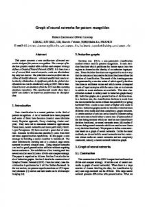
Figure 1: (a) Sample movement graph (Original graph). Each node is a stay point. (b) Summary of the same movement graph (Coarse graph). Each node represents a cluster of stay points.
safety and recommendation. In some applications (especially those related to prediction), the ability to accurately model the user movement is a make or break for good service provision. The efficient modeling of user’s mobility on a limited storage allows us to perform the mobility analysis algorithms on the smartphone that enhances the user’s experience. An intuitive approach is to model the movement of the user with a movement graph. The graph-based mobility models realize graphs in which nodes are the locations visited by the user and edge weights denote the distances or traveling times between locations. It should be noted that the movement graph can be defined in different ways. For example, Hsu et al. uses the weighted-way-point mobility model, in which the directed edges denote probabilities of choosing a destination based on the user current area [3]. Dealing with an original movement graph poses several challenges. First, the graph is usually large that cannot be fitted into the smartphone memory. In this case, the user’s movement cannot be analyzed on the smartphone device and need to be passed to the server, which reduces the reliability of the services. Second, due to the size of the graph, it is hard to visualize, understand and query the graph. Figure 1 (a) shows a sample movement graph of a student at RMIT University commuting between the library, shopping centre
and campus. Figure 1 (b) shows the same graph summarized and easy to understand where the edge weights denote the number of the movements. Furthermore, when the graph is big the queries are processed slowly, especially when running on a resource-limited device such as a smartphone. Third, the original graph is sparse and cannot be used for prediction. To build a machine learning model, we need sufficient data for training. However, if the graph is sparse, the model does not converge. For example, if we want to train the model for the next location prediction, we should have sufficient similar trajectories in the historical data for training. These challenges can be addressed by summarizing the movement graph to get a summarized graph where each node represents a cluster of nodes. In this paper, we exploit a new graph summarization method that is recently developed by partially the same authors as this paper [5]. The summarization is based on the iterative merging of the node pairs. In the summarized graph, known as the coarse graph, each node, called supernode, represents several nodes in the original graph. The edge weights in the coarse graph are defined in the way that the distances between the nodes are preserved. The coarse graph can be easily analyzed and stored in lower space. After summarizing the movement graph, we investigate its effect on two human mobility mining problems. First, we predict the location of the user based on the original and coarse graphs. We show that there is a trade-off between the granularity and accuracy of the results. Specifically, the prediction based on the coarse graph results in a better accuracy but the output is coarse-grain that includes several locations. Second, we study the effect of the summarization on computing the similarity between two movement graphs. To this end, we apply a graph similarity metric to both original and coarse graphs. As the coarse graph has fewer nodes, the summarization speeds up the calculation of similarity. However, if the compression ratio is too big, we lose information and the similarity cannot be calculated correctly. Summarization also addresses privacy issues as the exact location of the user cannot be determined in the coarse graph easily. Although in some situations, the user’s location can be still inferred, the location prediction generally becomes harder after summarization.
2.
RELATED WORK
Modeling the human mobility patterns with graphs is common in different analysis tasks such as location prediction, location inference, traffic anomaly detection, traveling time estimation, and most popular route detection [9]. The nodes in these graphs often are intersections or important locations (e.g. home or office), and the edges are road segments with traveling times as the weights. However, there are different ways to define the graph. In [8], the nodes are defined as regions and two nodes are connected with an edge if there is at least a certain number of commutes between them. Chen et al. extract the turning points from raw trajectory data and after clustering, they construct a graph that identifies the traveling probability to find the most popular route [1]. Zheng et al. construct a bipartite graph including users and locations for travel recommendation. In the graph, an edge between a user node and a location node exists if the user has visited the location [11]. Despite the vast usage of graphs in mobility mining, only a few researches use the summarized graph. Zheng et al. con-
Table 1: Summarization results for four users when the compression ratio is 10. #days Original Graph Coarse Graph Error nodes/edges supernodes/edges U1 466 117/298 12/22 4% U2 668 161/373 17/35 3% U3 454 81/140 9/16 6% U4 81 47/98 5/12 7%
struct hierarchical graphs from GPS trajectories to compute the similarity between different users. DB-Scan is deployed to cluster the GPS points and produce a hierarchical graph for each individual [10]. Although the hierarchical graphs include the summary graphs, their purpose is to use the summarized graph for friend and location recommendation. Our aim is to summarize the graph to be fitted in a lower storage space and to run the graph algorithms efficiently. There are many graph compression/summarization methods but only a few of them are applicable to our problem. Graph methods can be categorized into two groups: general compression and query-friendly compression. General compression methods use a specific property to preserve the information of the entire graph and answer all types of queries. These methods need decompression before querying the graph that is not suitable for our application where the compressed graph is stored and queried on a device. On the other hand, query-friendly compression approaches target specific classes of queries, such as neighborhood, pattern queries, connectivity, and distance-based queries [5]. Most of the compression methods target unweighted graphs such as web graphs and social networks and cannot be applied to weighted movement graphs.
3.
MOVEMENT GRAPH CONSTRUCTION
In this section, we describe the procedure of constructing the movement graph from a real-world dataset, Device Analyzer [7]. The Device Analyzer dataset includes data gathered from running background processes, wireless connectivity, GSM communication, and some system status and parameters. In this dataset, MAC addresses, Wifi SSIDs, and other forms of identification are hashed due to privacy purposes. As a result, there is no ground truth or information about the geography and semantic of the locations [7]. In our experiments, we extract the cell tower IDs (CIDs) connected to the smartphone. A CID is a labeled location whose geographical coordinates is unknown. To construct the movement graph, we start with identifying the stay points that can be defined in different ways. Based on our definition, a CID is considered as a stay point if the user is connected to it longer than one hour. A node is assigned to each stay point, and two nodes are connected if the user moves from one to the other stay point. The weight of the edge between the nodes denotes the traveling time from the time the user leaves the source stay point until he arrives at the destination one. If the user commutes between two nodes more than once, the mean values of traveling times is considered as the weight of the edge. A movement graph belongs to a user movement during a specific period. Table 1 shows the details of movement graphs extracted from Device Analyzer. The size of the graphs and the amount of the processed data are reported.
SUMMARIZATION
5.
SUMMARIZATION EFFECT
In this section, we show the effect of the summarization on two algorithms in terms of time, accuracy, and granularity.
5.1
Prediction
Here, the goal is to predict the location of the user based on the historical data and the time of the day. Specifically, we compute the probabilities of the presence of the user in all locations at a specific time of the day (e.g. 6 pm) by processing the historical data. Then, we choose the location with the highest probability as the location of the user. This method is one of the baselines for location prediction [2]. In our experiment, the Device Analyzer dataset is used where the locations are labeled with CIDs. After summarization, the prediction algorithm is applied to the coarse graph. The number of experimental instances is 1520 from 4 Device Analyzer users mentioned in Table 1. For each instance, the location of the user is predicted at a specific time that is identified by a supernode. If the predicted supernode in the coarse graph includes the actual CID that the user is connected to, the prediction is considered as successful. The accuracy is the number of successful predictions divided by the total number of experimental instances.
Historical data size (days)
0.9
Accuracy
After building the user’s movement graph, we apply Shrink to summarize the graph [5]. Shrink, applicable to a weighted graph, reduces the size of the graph by merging nodes while trying to preserve the distance between the nodes. After merging two nodes, a set of new weights are assigned to the edges connected to the nodes in the way that the distances have the least change. Hence, the distances between the nodes in the original and coarse graphs are almost the same. Therefore, to find the traveling distance between two CIDs, it is possible to run the shortest path algorithm on the coarse graph instead of the original graph. Each node in the coarse graph is a supernode representing a cluster of nodes from the original graph. Shrink is flexible about compression ratio (CR), which is the ratio of the number of nodes in the original graph to the number of nodes in the coarse graph. However, when the compression ratio is high, the distances are not preserved well. As the compression ratio is flexible, the user can set it based on the available storage. After storing the coarse graph, it can be queried without decompression. For any distance-based query such as shortest path query, the result is almost the same as running the query on the original graph. In our application, a supernode in the coarse graph represents a cluster of CIDs that may belong to a specific location such as university or shopping center. For example, assume several CIDs exist in the university and the user does not always connect to the same one. Shrink merges all the CIDs in the university to a supernode and updates its new edge weights. Table 1 reports the error when the compression ratio is equal to 10. The error is the average relative difference between the distances in the original and coarse graphs over 100 node pairs. The small value of the error indicates that the distances have been preserved well. We run our experiments on 4 different users containing 1689 days of data in total.
1.0
0.8
5 10
0.7
20 40
0.6
1
2
4
8
16
32
64
128
256
Compression Ratio
(a) 2.0
Historical data size (days)
1.5
Entropy
4.
5 1.0
10 20
0.5
40
0.0 1
2
4
8
16
32
64
128
256
Compression Ratio
(b) Figure 2: Effect of the summarization on the (a) accuracy of prediction (b) information gained by knowing the location of the user.
The compression ratio (CR) ranges from 1 to 256. CR equal to 1 indicates the case that no summarization is performed and the experiments run on the original graph. On the other hand, when CR is equal to 256, all of the nodes are merged into a single node and all information is lost. The length of the historical data ranges from 5 to 40 days. The accuracy is reported in Figure 2 (a).As it can be seen, when the compression ratio is high, the accuracy increases because the number of the possible locations for the user decreases which makes the prediction easier. In Figure 2 (b), Shannon entropy is reported. Intuitively, the entropy denotes the average amount of information gained by knowing the user’s location. From the figure, it can be seen that when the compression ratio increases, the entropy decrease as there are less possible locations. When CR is 256, we gain no information by knowing the user’s location as there is only one location (i.e. supernode). Furthermore, when the historical data is big, the number of CIDs visited by the user increases, the graph is larger, and the entropy is higher. Reporting the entropy is a proper way to measure how much privacy is lost by disclosing the user’s location.
5.2
Mining similarities
In this section, we show how the summarization changes the performance of the methods that measure the similarity between the movement graphs. Specifically, given two movement graphs of a user related to two different periods, the aim is to compute the similarity between the graphs. The result states how much the user’s mobility pattern changes over time, and it is based on the locations that the user visits and their frequencies. For example, let us consider a user that goes to the university every day but during the
100ms
10ms
1ms
1
2
4
8
16
32
64
128
256
Compression Ratio
Figure 3: Impact of the coarse graph size on the processing time required for measuring similarity. The dashed line shows when there is no summarization.
Similarities between coarse graphs
Processing Time
80
60
CR 2 4
40
8
20
0 25
50
75
Similarities between original graphs
exam period, he goes to the library to study. By building the movement graph in exam period and comparing it with user’s normal movement graph, we can detect when the user’s mobility pattern changes [4]. In our experiments, we deploy Graph Edit Distance (GED) to measure the similarity between two graphs [6]. Using this approach, the dissimilarity between two graphs is defined as the minimum number of operations required to convert one graph to the other. The operations include edge insertion/removal, node insertion/removal, and increasing/ decreasing an edge weight. Figure 3 shows the effect of the summarization on the processing time for the GED algorithm. When the compression ratio is high, the coarse graph has fewer nodes. Consequently, comparing the graphs is performed faster. In Figure 4, we show that comparing the coarse graphs is almost the same as comparing the original graphs. In fact, the summarization has a little effect on the GED results and if two graphs are similar/dissimilar, after the summarization, the similarity/dissimilarity remains the same. However, by increasing the compression ratio, the uncertainty is increased too. For CR=2, the Pearson correlation coefficient is 0.98 but when the compression ratio becomes bigger, the correlation decreases. To sum up, by increasing the compression ratio, the processing time of GED algorithm decreases but at the same time, the uncertainty of the result increases, which means the results is less reliable.
6.
CONCLUSION AND FUTURE WORK
The movement graph is useful in many problems regarding the user mobility pattern such as location prediction and mining changes in the mobility pattern. We obtain a coarse graph from the original movement graph that includes the locations visited by the user and transitions between them. The coarse graph is an abstract representation of the original graph. We also investigate the effect of using the coarse graph rather than the original graph on two algorithms. From the experiment result, it can be inferred that mining the coarse graph is faster but less accurate. This creates a trade-off between accuracy, storage space, and speed that can be controlled by the compression ratio. In addition to the efficiency, summarization is desirable for privacy issues because each node of the graph reveals less information about the user’s location.
Figure 4: By increasing the compression ratio (CR), the correlation decreases.
7.
REFERENCES
[1] Z. Chen, H. T. Shen, and X. Zhou. Discovering popular routes from trajectories. In (ICDE), pages 900–911. IEEE, 2011. [2] T. M. T. Do, O. Dousse, M. Miettinen, and D. Gatica-Perez. A probabilistic kernel method for human mobility prediction with smartphones. Pervasive and Mobile Computing, 20:13–28, 2015. [3] W.-j. Hsu, K. Merchant, H.-w. Shu, C.-h. Hsu, and A. Helmy. Weighted waypoint mobility model and its impact on ad hoc networks. ACM SIGMOBILE Mobile Computing and Communications Review, 9(1):59–63, 2005. [4] A. Sadri. Mining changes in mobility patterns from smartphone data. In PerCom Workshops, pages 1–3. IEEE, 2016. [5] A. Sadri, F. D. Salim, Y. Ren, M. Zameni, J. Chan, and T. Sellis. Shrink: Distance preserving graph compression. Information Systems, 2017. [6] A. Sanfeliu and K.-S. Fu. A distance measure between attributed relational graphs for pattern recognition. IEEE transactions on systems, man, and cybernetics, (3):353–362, 1983. [7] D. T. Wagner, A. Rice, and A. R. Beresford. Device analyzer: Large-scale mobile data collection. ACM SIGMETRICS, 41(4):53–56, 2014. [8] J. Yuan, Y. Zheng, and X. Xie. Discovering regions of different functions in a city using human mobility and pois. In SIGKDD, pages 186–194. ACM, 2012. [9] Y. Zheng. Trajectory data mining: an overview. ACM Transactions on Intelligent Systems and Technology (TIST), 6(3):29, 2015. [10] Y. Zheng, L. Zhang, Z. Ma, X. Xie, and W.-Y. Ma. Recommending friends and locations based on individual location history. ACM Transactions on the Web (TWEB), 5(1):5, 2011. [11] Y. Zheng, L. Zhang, X. Xie, and W.-Y. Ma. Mining interesting locations and travel sequences from gps trajectories. In WWW, pages 791–800. ACM, 2009.