Hindawi Publishing Corporation e Scientific World Journal Volume 2014, Article ID 840185, 10 pages http://dx.doi.org/10.1155/2014/840185
Research Article Synchronization Control for Stochastic Neural Networks with Mixed Time-Varying Delays Qing Zhu,1,2 Aiguo Song,1 Shumin Fei,3 Yuequan Yang,2 and Zhiqiang Cao4 1
School of Instrument Science, Southeast University, Nanjing 210096, China College of Information Engineering, Yangzhou University, Yangzhou 225009, China 3 School of Automation, Southeast University, Nanjing 210096, China 4 Institute of Automation, Chinese Academy of Science, Beijing 100190, China 2
Correspondence should be addressed to Aiguo Song;
[email protected] Received 18 May 2014; Accepted 7 June 2014; Published 2 July 2014 Academic Editor: Guanghui Wen Copyright © 2014 Qing Zhu et al. This is an open access article distributed under the Creative Commons Attribution License, which permits unrestricted use, distribution, and reproduction in any medium, provided the original work is properly cited. Synchronization control of stochastic neural networks with time-varying discrete and continuous delays has been investigated. A novel control scheme is proposed using the Lyapunov functional method and linear matrix inequality (LMI) approach. Sufficient conditions have been derived to ensure the global asymptotical mean-square stability for the error system, and thus the drive system synchronizes with the response system. Also, the control gain matrix can be obtained. With these effective methods, synchronization can be achieved. Simulation results are presented to show the effectiveness of the theoretical results.
1. Introduction In recent years, stochastic neural networks (NNs) have gained particular research interests. These systems represent a class of stochastic systems that is popular in modeling practical systems which may experience random disturbances and parameters varying. Such a system can be found in biology systems, social systems, and wireless communication networks. Numerous results on stochastic neural network have been reported in the literature [1–5]. As one of the mostly investigated dynamical behaviors, the synchronization in stochastic NNs with or without time delays has drawn significant research interest; see, for example, [6–10] and the references therein. On the other hand, time delays are frequently encountered in many practical control systems, such as aircraft, chemical, or process control systems. The existence of the time delays may be the source of instability of serious deterioration in the performance of the closed-loop systems. Thus, stability of delayed NNs has been a focal subject for research [11–15]. Most recently, significant and substantial progresses have been achieved in the synchronization of
stochastic NNs. These include synchronization of randomly coupled neural networks with Markovian jumping and timedelay [15], adaptive synchronization for stochastic NNs with time-varying delays and distributed delays [16], passivity analysis for discrete time stochastic Markovian jump NNs with mixed time delays [17], adaptive synchronization for stochastic T-S fuzzy NNs with time-delay and Markovian jumping parameters [18], nonfragile synchronization of NNs with time-varying delay and randomly occurring controller gain fluctuation synchronization of biological NN systems with stochastic perturbations and time delays [19], global exponential adaptive synchronization of complex dynamical networks with neutral-type NN nodes and stochastic disturbances [20], adaptive synchronization for uncertain chaotic neural networks with mixed time delays using fuzzy disturbance observer [21], the effects of time delay on the stochastic resonance in feed-forward-loop NN motifs [22], state estimation for wireless network control system with stochastic uncertainty and time delay based on sliding mode observer [23], pinning synchronization in fixed and switching directed networks of Lorenz-type nodes [24], consensus tracking for higher-order multiagent systems with switching directed
2
The Scientific World Journal
topologies and occasionally missing control inputs [25], and consensus tracking of multiagent systems with Lipschitz-type node dynamics and switching topologies [26]. Although substantial progresses have been made in the synchronization control of delayed stochastic neural network systems [16–32], there are still some problems which have not been fully studied. For example, many control schemes of time-varying delayed NNs assume that the derivative of the time-delay function is less than one. Also, few works have been done on the synchronization of mixed delayed stochastic NNs. In this paper, we propose sufficient conditions of the synchronization of the stochastic NN system, as well as the state feedback control design. At first, sufficient conditions are proposed in terms of LMIs to guarantee the stochastic asymptotical stability of the error system. The assumption that the derivative of the time-delay function is less than one is eliminated. Then, we give some corollaries to solve the problem in some special cases. This paper is organized as follows. After the introduction in Section 1, the problem statement and preliminaries are presented in Section 2. Next, some sufficient conditions are presented for the synchronization of the delayed drive and response system. Also, some corollaries and remarks are given to show the advantages of this paper in Section 3. Then, the numerical simulation result is given in Section 4. A conclusion is drawn in Section 5.
2. Problem Statement and Preliminaries Before proceeding, we introduce some notations which will be used later for derivations and discussions. ‖ ⋅ ‖ denotes the Euclidean norm of a vector or the Frobenius norm of a matrix. 𝑀 > 0 ( 0: 𝑓𝑖 (𝑥) − 𝑓𝑖 (𝑦) ≤ 𝑘𝑖 𝑥 − 𝑦
∀𝑥, 𝑦 ∈ 𝑅, 𝑖 = 1, 2, . . . , 𝑛,
𝐾 = diag (𝑘1 , 𝑘2 , . . . , 𝑘𝑛 ) . (3) (A2) Matrix function 𝜎(𝑡, 𝑒(𝑡), 𝑒(𝑡 − 𝜏(𝑡))) satisfies trace [𝜎𝑇 (𝑡, 𝑒 (𝑡) , 𝑒 (𝑡 − 𝜏 (𝑡))) 𝜎 (𝑡, 𝑒 (𝑡) , 𝑒 (𝑡 − 𝜏 (𝑡)))] (4) 2 2 ≤ 𝑀1 𝑒 (𝑡) + 𝑀2 𝑒(𝑡 − 𝜏(𝑡)) , where 𝑀1 and 𝑀2 are matrices with appropriate dimensions. (A3) Discrete delay 𝜏(𝑡) and continuous delay 𝜎(𝑡) are both differential functions of time, and the following conditions hold: 𝜏̇ (𝑡) ≤ 𝜏1 ,
0 ≤ 𝜏 (𝑡) ≤ 𝜏,
0 ≤ 𝜎 (𝑡) ≤ 𝜎,
(5)
where 𝜏, 𝜏1 , and 𝜎 are positive constants. It is worth to emphasis that the constraint, the derivative of time-delay function is less than one [1], is eliminated in this paper, while a more general upper boundary constraint is utilized instead of it. This improvement makes our results applicable for a wide range of time-delayed stochastic neural networks. Let error state be 𝑒(𝑡) = 𝑦(𝑡)−𝑥(𝑡); subtracting (1) from (2) yields the synchronization error dynamical system as follows: 𝑑𝑒 (𝑡) = [ − 𝐶𝑒 (𝑡) + 𝐴𝑔 (𝑡) + 𝐵𝑔 (𝑡 − 𝜏 (𝑡)) 𝑡
+𝐷 ∫
𝑡−𝜎(𝑡)
𝑔 (𝑠) 𝑑𝑠 + 𝑢 (𝑡)] 𝑑𝑡
(6)
+ 𝜎 (𝑡, 𝑒 (𝑡) , 𝑒 (𝑡 − 𝜏 (𝑡))) 𝑑𝜔, where 𝑔(𝑡) = 𝑓(𝑦(𝑡)) − 𝑓(𝑥(𝑡)). In this paper, we design a memoryless state feedback controller: 𝑢 (𝑡) = 𝐺𝑒 (𝑡) , where 𝐺 ∈ 𝑅𝑛×𝑛 is a constant gain matrix.
(7)
The Scientific World Journal
3
Substituting the controller into the error system (6), we get
𝑑𝑒 (𝑡) = [ (−𝐶 + 𝐺) 𝑒 (𝑡) + 𝐴𝑔 (𝑡) + 𝐵𝑔 (𝑡 − 𝜏 (𝑡)) +𝐷 ∫
𝑡
𝑡−𝜎(𝑡)
Definition 1. The system (8) is called globally asymptotically mean-square stable, if the following holds:
for any 𝑒 (𝑡0 ) ,
(9)
where 𝐸⋅ is the mathematical expectation. The following Lemma is given. Lemma 2 (Schur complement lemma). For matrices 𝐴, 𝐵, and 𝐶 with compatible dimensions, the following three conditions are equivalent: Π11 𝑄1 Π13
[
𝐴 − 𝐶𝐵−1 𝐶𝑇 < 0,
𝐵 < 0,
if B is invertible; (11)
(c)
𝐵 − 𝐶𝑇 𝐴−1 𝐶 < 0,
𝐴 < 0,
if A is invertible. (12)
0
𝑏
𝑏
𝑏
𝑎
𝑎
𝑎
∫ 𝑓𝑇 (𝑡) 𝑑𝑡 𝑃 ∫ 𝑓 (𝑡) 𝑑𝑡 ≤ (𝑏 − 𝑎) ∫ 𝑓𝑇 (𝑡) 𝑃𝑓 (𝑡) 𝑑𝑡. (13)
It is well known that system (8) has a unique solution [33].
[ [ [ [ [ [ [ [ [ [ Π= [ [ [ [ [ [ [ [ [ [
(b)
(10)
Lemma 3. For vector function 𝑓(𝑡) ∈ 𝑅𝑛 and symmetric matrix 𝑃 > 0, the following holds:
+ 𝜎 (𝑡, 𝑒 (𝑡) , 𝑒 (𝑡 − 𝜏 (𝑡))) 𝑑𝜔.
lim 𝐸‖𝑒 (𝑡)‖2 = 0,
[
(8)
𝑔 (𝑠) 𝑑𝑠] 𝑑𝑡
𝑡→∞
𝐴 𝐶 ] < 0; 𝐶𝑇 𝐵
(a)
3. Criteria of Synchronization In this section, new criteria are presented for the global asymptotical stability of the equilibrium point of the neural network defined by (8), and thus the drive system (1) synchronizes with the response system (2). Its proof is based on a new Lyapunov functional method and linear matrix inequality (LMI) approach. Theorem 4. Under the assumptions A1–A3, the equilibrium point of model (8) is called globally asymptotically stable in mean-square, if there exist symmetric positive-definite matrices 𝑃𝑗 ( 𝑗 = 1, . . . , 4), diagonal matrices 𝐷1 , 𝐷2 , and general matrix 𝑄1 such that the following inequalities hold:
Π14
0
𝑃1 𝐷 + 𝜏2 𝐷
𝜏(−𝐶 + 𝐺)𝑇 𝑃1
𝐾𝑇 𝐷2
−𝑄1
0
0
0
𝜏2 𝐴𝑇 𝑃1 𝐷
0
∗
Π22
∗
∗
∗
∗
∗
Π44
0
𝜏2 𝐵𝑇 𝑃1 𝐷
0
∗
∗
∗
∗
−𝑃1
0
0
∗
∗
∗
∗
∗
−𝑃4 + 𝜏2 𝐷𝑇 𝑃1 𝐷
0
∗
∗
∗
∗
∗
∗
−𝑃1
Π33 𝜏2 𝐴𝑇 𝑃1 𝐵
] ] ] ] ] ] ] ] ] ] ] < 0, ] ] ] ] ] ] ] ] ]
(14)
]
𝑃1 < 𝜌𝐼,
(15)
Π33 = 𝑃3 − 2𝐷1 + 𝜎2 𝑃4 + 𝜏2 𝐴𝑇 𝑃1 𝐴,
where Π11 = 𝑃1 (−𝐶 + 𝐺) + (−𝐶 + 𝐺)𝑇 𝑃1 + 𝑃2 + 𝜌𝑀1𝑇 𝑀1 ,
Π44 = − (1 − 𝜏1 ) 𝑃3 − 2𝐷2 + 𝜏2 𝐵𝑇 𝑃1 𝐵. (16)
Π13 = 𝑃1 𝐴 + 𝐾𝑇𝐷1 + 𝜏2 (−𝐶 + 𝐺)𝑇 𝑃1 𝐴, 2
Proof. The Lyapunov function candidate is given as
𝑇
Π14 = 𝑃1 𝐵 + 𝜏 (−𝐶 + 𝐺) 𝑃1 𝐵, Π22 = − (1 − 𝜏1 ) 𝑃2 − 𝑄1 − 𝑄1𝑇 + 𝜌𝑀2𝑇 𝑀2 ,
5
𝑉 (𝑡) = ∑ 𝑉𝑖 (𝑡) , 𝑖=1
(17)
4
The Scientific World Journal
where
By Lemma 3, we obtain 𝑉1 (𝑡) = 𝑒𝑇 (𝑡) 𝑃1 𝑒 (𝑡) , 𝑉2 (𝑡) = ∫
𝑡
𝑡−𝜏(𝑡)
𝑉3 (𝑡) = ∫
𝑡
𝑡−𝜏(𝑡)
− 𝜏∫
𝑡−𝜏
𝑒𝑇 (𝑠) 𝑃2 𝑒 (𝑠) 𝑑𝑠,
𝑒𝑇̇ (𝑠) 𝑃1 𝑒 ̇ (𝑠) 𝑑𝑠
≤ −𝜏 (𝑡) ∫
𝑡
𝑡−𝜏(𝑡)
𝑔𝑇 (𝑠) 𝑃3 𝑔 (𝑠) 𝑑𝑠,
≤ −∫
𝑡
𝜏
𝑡
0
𝑡−𝑠
− 𝜎∫
𝑡
𝑡−𝜎
𝑡
𝑉5 (𝑡) = 𝜎 ∫ ∫ 𝑔𝑇 (𝜃) 𝑃4 𝑔 (𝜃) 𝑑𝜃 𝑑𝑠.
𝑡
𝑡−𝜎(𝑡)
𝑡
𝑡−𝜎(𝑡)
≤ −∫
𝑡
𝑡−𝜎(𝑡)
𝑔𝑇 (𝑠) 𝑃4 𝑔 (𝑠) 𝑑𝑠
𝑔𝑇 (𝑠) 𝑑𝑠 𝑃4 ∫
𝑡
𝑡−𝜎(𝑡)
𝑒 (𝑡) − 𝑒 (𝑡 − 𝜏 (𝑡)) = ∫
𝑡
𝑡−𝜏(𝑡)
𝑔 (𝑠) 𝑑𝑠]
(19)
𝑒 ̇ (𝑠) 𝑑𝑠,
(26)
𝑔 (𝑠) 𝑑𝑠.
By Newton-Leibniz formula, we have
L𝑉1 = 2𝑒𝑇 (𝑡) 𝑃1 [ (−𝐶 + 𝐺) 𝑒 (𝑡) + 𝐴𝑔 (𝑡) +𝐵𝑔 (𝑡 − 𝜏 (𝑡)) + 𝐷 ∫
(25)
𝑔𝑇 (𝑠) 𝑃4 𝑔 (𝑠) 𝑑𝑠
(18) The weak infinitesimal operator 𝐿 of the process {𝑥𝑡 = 𝑥(𝑡 + 𝑠), 𝑡 ≥ 0, −𝜏 ≤ 𝑡 ≤ 0} is given by
𝑡
𝑡−𝜏(𝑡)
≤ −𝜎 (𝑡) ∫
−𝜎 𝑡+𝑠
𝑒𝑇̇ (𝑠) 𝑃1 𝑒 ̇ (𝑠) 𝑑𝑠
𝑒𝑇̇ (𝑠) 𝑑𝑠 𝑃1 ∫
𝑡−𝜏(𝑡)
𝑉4 (𝑡) = 𝜏 ∫ ∫ 𝑒𝑇̇ (𝜃) 𝑃1 𝑒 ̇ (𝜃) 𝑑𝜃 𝑑𝑠, 0
𝑡
𝑒 ̇ (𝑠) 𝑑𝑠.
(27)
From assumption A1, we get 𝑔𝑇 (𝑡) 𝐷1 𝑔 (𝑡) ≤ 𝑔𝑇 (𝑡) 𝐷1 𝐾𝑒 (𝑡) ,
+ trace [𝜎𝑇 (𝑡, 𝑒 (𝑡) , 𝑒 (𝑡 − 𝜏 (𝑡)))
𝑔𝑇 (𝑡 − 𝜏 (𝑡)) 𝐷2 𝑔 (𝑡 − 𝜏 (𝑡)) ≤ 𝑔𝑇 (𝑡 − 𝜏 (𝑡)) 𝐷2 𝐾𝑒 (𝑡 − 𝜏 (𝑡)) , (28)
× 𝑃1 𝜎 (𝑡, 𝑒 (𝑡) , 𝑒 (𝑡 − 𝜏 (𝑡))) ] .
where 𝐾, 𝐷1 , and 𝐷2 are positive-definite diagonal matrices. By (27) and (28), we define several nonnegative expressions as follows:
By (5) and (14), we have trace [𝜎𝑇 (𝑡, 𝑒 (𝑡) , 𝑒 (𝑡 − 𝜏 (𝑡)))
𝑡
𝐿1 = 2𝑒 (𝑡 − 𝜏 (𝑡)) 𝑄1 [𝑒 (𝑡) − 𝑒 (𝑡 − 𝜏 (𝑡)) − ∫
× 𝑃1 𝜎 (𝑡, 𝑒 (𝑡) , 𝑒 (𝑡 − 𝜏 (𝑡))) ]
𝑡−𝜏(𝑡)
𝑒 ̇ (𝑠) 𝑑𝑠]
= 0,
≤ 𝜌 trace [𝜎𝑇 (𝑡, 𝑒 (𝑡) , 𝑒 (𝑡 − 𝜏 (𝑡)))
(29)
(20) × 𝜎 (𝑡, 𝑒 (𝑡) , 𝑒 (𝑡 − 𝜏 (𝑡))) ]
𝐿2 = 2 [𝑔𝑇 (𝑡) 𝐷1 𝐾𝑒 (𝑡) − 𝑔𝑇 (𝑡) 𝐷1 𝑔 (𝑡)] ≥ 0,
= 𝜌 [𝑒𝑇 (𝑡) 𝑀1𝑇 𝑀1 𝑒 (𝑡)
𝐿3 = 2 [𝑔𝑇 (𝑡 − 𝜏 (𝑡)) 𝐷2 𝐾𝑒 (𝑡 − 𝜏 (𝑡)) − 𝑔𝑇 (𝑡 − 𝜏 (𝑡))
+𝑒𝑇 (𝑡 − 𝜏 (𝑡)) 𝑀2𝑇 𝑀2 𝑒 (𝑡 − 𝜏 (𝑡))] , 𝐿𝑉2 (𝑡) = 𝑒𝑇 (𝑡) 𝑃2 𝑒 (𝑡) − (1 − 𝜏̇ (𝑡)) 𝑒𝑇 × (𝑡 − 𝜏 (𝑡)) 𝑃2 𝑒 (𝑡 − 𝜏 (𝑡)) , 𝐿𝑉3 (𝑡) = 𝑔𝑇 (𝑡) 𝑃3 𝑔 (𝑡) − (1 − 𝜏̇ (𝑡)) 𝑔𝑇 × (𝑡 − 𝜏 (𝑡)) 𝑃3 𝑔 (𝑡 − 𝜏 (𝑡)) , 𝐿𝑉4 (𝑡) = 𝜏2 𝑒𝑇̇ (𝑡) 𝑃1 𝑒 ̇ (𝑡) − 𝜏 ∫
𝑡
𝑡−𝜏
2 𝑇
𝐿𝑉5 (𝑡) = 𝜎 𝑔 (𝑡) 𝑃4 𝑔 (𝑡) − 𝜎 ∫
𝑡
𝑡−𝜎
𝑒𝑇̇ (𝑠) 𝑃1 𝑒 ̇ (𝑠) 𝑑𝑠, 𝑇
𝑔 (𝑠) 𝑃4 𝑔 (𝑠) 𝑑𝑠.
×𝐷2 𝑔 (𝑡 − 𝜏 (𝑡)) ] ≥ 0. (21)
(22)
(30) (31)
Then expressions 𝐿1, 𝐿2, and 𝐿3 are to be added to the inequality of 𝐿𝑉(𝑡) to facilitate the proof. Therefore, combining (19)–(29) we have 5
𝐿𝑉 (𝑡) ≤ ∑ 𝐿𝑉𝑖 (𝑡) + 𝐿1 + 𝐿2 + 𝐿3 𝑖=1
(23) (24)
≤ 𝑒𝑇 (𝑡) [2𝑃1 (−𝐶 + 𝐺) + 𝜌𝑀1𝑇 𝑀1 + 𝑃2 ] 𝑒 (𝑡) + 𝑒𝑇 (𝑡 − 𝜏 (𝑡)) [− (1 − 𝜏1 ) 𝑃2 + 𝜌𝑀2𝑇 𝑀2 − 2𝑄1 ] × 𝑒 (𝑡 − 𝜏 (𝑡))
The Scientific World Journal
5
+ 𝑔𝑇 (𝑡) [𝑃3 − 2𝐷1 + 𝜎2 𝑃4 ] 𝑔 (𝑡)
We introduce matrices 𝑀 and 𝐻 which satisfy
𝑇
+ 𝑔 (𝑡 − 𝜏 (𝑡)) [− (1 − 𝜏1 ) 𝑃3 − 2𝐷2 ] 𝑔 (𝑡 − 𝜏 (𝑡)) 𝑡
𝑡
−∫
𝑒𝑇̇ (𝑠) 𝑑𝑠 𝑃1 ∫
−∫
𝑔𝑇 (𝜃) 𝑑𝜃 𝑃4 ∫
𝑡−𝜏 𝑡 𝑡−𝜎
𝑡−𝜏 𝑡
Π=[
𝑒 ̇ (𝑠) 𝑑𝑠
𝑡−𝜎
𝑀 𝐻 ], 𝐻𝑇 −𝑃1
−1
𝑁 = 𝑀 − 𝐻(−𝑃1 ) 𝐻𝑇 ,
(34)
𝑔 (𝜃) 𝑑𝜃 where
𝑇
+ 2𝑒 (𝑡) 𝑄1 𝑒 (𝑡 − 𝜏 (𝑡)) + 𝑒𝑇 (𝑡) [2𝑃1 𝐴 + 2𝐾𝑇 𝐷1 ] 𝑔 (𝑡)
[ [ [ [ [ [ [ [ 𝑀= [ [ [ [ [ [ [ [
𝑇
+ 2𝑒 (𝑡) [𝑃1 𝐵] 𝑔 (𝑡 − 𝜏 (𝑡)) 𝑇
+ 2𝑒 (𝑡) [𝑃1 𝐷] ∫
𝑡
𝑡−𝜎(𝑡)
𝑔 (𝜃) 𝑑𝜃
+ 2𝑒𝑇 (𝑡 − 𝜏 (𝑡)) [𝐾𝑇 𝐷2 ] 𝑔 (𝑡 − 𝜏 (𝑡)) + 2𝑒𝑇 (𝑡 − 𝜏 (𝑡)) [𝑄1 ] ∫
𝑡
𝑡−𝜏
𝑒 ̇ (𝑠) 𝑑𝑠
[
𝑡
𝑡−𝜎(𝑡)
× 𝜏2 𝑃1 [ (−𝐶 + 𝐺) 𝑒 (𝑡) + 𝐴𝑔 (𝑡)
𝑡−𝜎(𝑡)
𝑃1 𝐷 + 𝜏2 𝐷
𝐾𝑇𝐷2
−𝑄1
0
0
𝜏2 𝐴𝑇 𝑃1 𝐷
∗
Π22
∗
∗
∗
∗
∗
Π44
0
𝜏2 𝐵𝑇 𝑃1 𝐷
∗
∗
∗
∗
−𝑃1
0
∗
∗
∗
∗
∗
−𝑃4 + 𝜏2 𝐷𝑇 𝑃1 𝐷
0
Π33 𝜏2 𝐴𝑇 𝑃1 𝐵
𝜏(−𝐶 + 𝐺) 𝑃1 ] 0 ] ] 0 ]. ] 0 ] ] 0 0 ] [
𝑇
𝑡
0
(32)
(35)
𝑡
𝐸𝑉 (𝑡) − 𝐸𝑉 (𝑡0 ) = 𝐸 ∫ 𝐿𝑉 (𝑠) 𝑑𝑠. 𝑡0
where 𝜉 = [𝑒𝑇 (𝑡) , 𝑒𝑇 (𝑡 − 𝜏 (𝑡)) , 𝑔𝑇 (𝑡) , 𝑔𝑇 (𝑡 − 𝜏 (𝑡)) , 𝑡
𝑡−𝜏(𝑡)
𝑒𝑇̇ (𝑠) 𝑑𝑠, ∫
𝑡
𝑡−𝜎(𝑡)
]
By Lemma 2, we get that Π < 0 ⇔ 𝑁 < 0, −𝑃1 < 0. Thus 𝐿𝑉 < 0. From (24) and the Ito formula, it is obvious that
𝑔 (𝑠) 𝑑𝑠]
≤ 𝜉𝑇 𝑁𝜉,
∫
] ] ] ] ] ] ] ] ], ] ] ] ] ] ] ]
[ [ [ 𝐻= [ [ [ [
𝑔 (𝑠) 𝑑𝑠]
+𝐵𝑔 (𝑡 − 𝜏 (𝑡)) + 𝐷 ∫
Π14
𝑇
+ [ (−𝐶 + 𝐺) 𝑒 (𝑡) + 𝐴𝑔 (𝑡) + 𝐵𝑔 (𝑡 − 𝜏 (𝑡)) +𝐷∫
Π11 𝑄1 Π13
(36)
From the definition of 𝑉(𝑡) in (15), there exists positive constant 𝜆 1 such that
𝑇
𝑔𝑇 (𝑠) 𝑑𝑠] ,
𝑡
Π14 0 𝑃1 𝐷 + 𝜏2 𝐷 𝑁11 𝑄1 Π13 ] [ ] [ ∗ Π22 0 𝐾𝑇𝐷2 −𝑄1 0 ] [ ] [ ] [ 2 𝑇 2 𝑇 ] [∗ ∗ Π 𝜏 𝐴 𝑃 𝐵 0 𝜏 𝐴 𝑃 𝐷 33 1 1 ] [ ] [ 𝑁=[ ], [∗ ∗ ∗ Π44 0 𝜏2 𝐵𝑇 𝑃1 𝐷 ] ] [ ] [ ] [∗ ∗ ∗ ∗ −𝑃1 0 ] [ ] [ ] [ 2 𝑇 ∗ ∗ ∗ ∗ ∗ −𝑃4 + 𝜏 𝐷 𝑃1 𝐷 ] [ 𝑇 𝑁11 = 𝑃1 (−𝐶 + 𝐺) + (−𝐶 + 𝐺) 𝑃1 + 𝑃2 + 𝜌𝑀1𝑇 𝑀1 + 𝜏2 (−𝐶 + 𝐺)𝑇 𝑃1 (−𝐶 + 𝐺) . (33)
𝜆 1 𝐸‖𝑒(𝑡)‖2 ≤ 𝐸𝑉 (𝑡) ≤ 𝐸𝑉 (𝑡0 ) + 𝐸 ∫ 𝐿𝑉 (𝑠) 𝑑𝑠 𝑡0
𝑡
(37) 2
≤ 𝐸𝑉 (𝑡0 ) + 𝜆 max 𝐸 ∫ ‖𝑒(𝑠)‖ 𝑑𝑠, 𝑡0
where 𝜆 max is the maximal eigenvalue of 𝑁 and it is negative. Therefore, from (26) and the discussion in [34], we know that the equilibrium of (11) is globally asymptotically stable in mean-square. This completes the proof. Corollary 5. Under the assumptions A1–A3, the equilibrium point of model (8) is called globally asymptotically stable in mean-square, if there exist symmetric positive-definite matrices 𝑃𝑗 (𝑗 = 1, . . . , 4), diagonal matrices 𝐷1 , 𝐷2 , and general matrices 𝑄1 and 𝑊, such that the following inequalities hold:
6
The Scientific World Journal
[ [ [ [ [ [ [ [ [ [ Π= [ [ [ [ [ [ [ [ [ [ [
∗
Π22
0
∗
∗
Π33
∗
∗
∗
∗
∗
∗
∗
∗
∗
∗
∗
∗
𝑃1 𝐷 + 𝜏2 𝐷
𝜏 (−𝐶𝑇 𝑃1 + 𝑊𝑇 ) ] ] 𝐾𝑇𝐷2 −𝑄1 0 0 ] ] ] 2 𝑇 2 𝑇 ] 𝜏 𝐴 𝑃1 𝐵 0 𝜏 𝐴 𝑃1 𝐷 0 ] ] ] 2 𝑇 ] Π44 0 𝜏 𝐵 𝑃1 𝐷 0 ] < 0, ] ] ] ∗ −𝑃1 0 0 ] ] ] 2 𝑇 ∗ ∗ −𝑃4 + 𝜏 𝐷 𝑃1 𝐷 0 ] ] ] ∗ ∗ ∗ −𝑃1 ]
Π11 𝑄1 Π13
Π14
0
(38)
𝑃1 < 𝜌𝐼,
Furthermore, the control gain matrix 𝐺 is given as
where Π11 = − 𝑃1 𝐶 − 𝐶𝑇 𝑃1 + 𝑊 + 𝑊𝑇 + 𝑃2 + 𝜌𝑀1𝑇 𝑀1 , 𝑇
2
𝑇
𝐺 = 𝑃1−1 𝑊.
𝑇
Π13 = 𝑃1 𝐴 + 𝐾 𝐷1 + 𝜏 (−𝐶 𝑃1 + 𝑊 ) 𝐴, 2
𝑇
(40)
Proof. Let 𝑊 = 𝑃1 𝐺 in Theorem 4; it is easy to get the result.
𝑇
Π14 = 𝑃1 𝐵 + 𝜏 (−𝐶 𝑃1 + 𝑊 ) 𝐵, Π22 = − (1 − 𝜏1 ) 𝑃2 − 𝑄1 − 𝑄1𝑇 + 𝜌𝑀2𝑇 𝑀2 , Π33 = 𝑃3 − 2𝐷1 + 𝜎2 𝑃4 + 𝜏2 𝐴𝑇 𝑃1 𝐴, Π44 = − (1 − 𝜏1 ) 𝑃3 − 2𝐷2 + 𝜏2 𝐵𝑇 𝑃1 𝐵. (39)
[ [ [ [ [ [ [ [ [ Π= [ [ [ [ [ [ [ [ [ [
Π11 𝑄1 Π13
[ 𝑃1 < 𝜌𝐼,
∗
Π22
0
∗
∗
Π33
∗
∗
∗
∗
∗
∗
∗
∗
∗
∗
∗
∗
Corollary 6. If the systems (1) and (2) have no integral timedelay items (e.g., 𝐷 = 0), the result can be simplified as follows. Under assumptions A1–A3 and 𝐷 = 0, the equilibrium point of model (8) is called globally asymptotically stable in mean-square, if there exist symmetric positive-definite matrices 𝑃𝑗 (𝑗 = 1, . . . , 4), diagonal matrices 𝐷1 , 𝐷2 , and general matrices 𝑄1 and 𝑊, such that the following inequalities hold:
𝜏 (−𝐶𝑇 𝑃1 + 𝑊𝑇 ) ] ] 𝐾𝑇𝐷2 −𝑄1 0 ] ] ] 2 𝑇 ] 𝜏 𝐴 𝑃1 𝐵 0 0 ] ] ] 0 0 Π44 ] < 0, ] ] ] ∗ −𝑃1 0 ] ] ] ] ∗ ∗ 0 ] ] ∗ ∗ −𝑃1 ] Π14
0
(41)
Π22 = − (1 − 𝜏1 ) 𝑃2 − 𝑄1 − 𝑄1𝑇 + 𝜌𝑀2𝑇 𝑀2 ,
where 𝑇
𝑇
Π11 = − 𝑃1 𝐶 − 𝐶 𝑃1 + 𝑊 + 𝑊 + 𝑃2 + 𝑇
2
𝑇
𝑇
𝜌𝑀1𝑇 𝑀1 ,
Π13 = 𝑃1 𝐴 + 𝐾 𝐷1 + 𝜏 (−𝐶 𝑃1 + 𝑊 ) 𝐴, Π14 = 𝑃1 𝐵 + 𝜏2 (−𝐶𝑇 𝑃1 + 𝑊𝑇 ) 𝐵,
Π33 = 𝑃3 − 2𝐷1 + 𝜎2 𝑃4 + 𝜏2 𝐴𝑇 𝑃1 𝐴,
(42)
2 𝑇
Π44 = − (1 − 𝜏1 ) 𝑃3 − 2𝐷2 + 𝜏 𝐵 𝑃1 𝐵. Furthermore, the control gain matrix 𝐺 is given as 𝐺 = 𝑃1−1 𝑊.
(43)
The Scientific World Journal
7
5
0.8
4
0.6
3
0.4
2
0.2
x2
x1
1 0
0 −0.2
−1
−0.4
−2 −3
−0.6
−4
−0.8
−5 −1
−0.8 −0.6 −0.4 −0.2
0 x1
0.2
0.4
0.6
0.8
−1
1
20
0
40
60
80
5
5
4
4
3
3
2
2
1
1
0
0
x2
y2
120
140 160
180
200
100 t
120
140 160
180
200
(a)
(a)
−1
−1
−2
−2
−3
−3
−4
−4
−5 −1 −0.8 −0.6 −0.4 −0.2
100 t
0
0.2
0.4
0.6
0.8
1
−5
20
0
40
60
80
y1 (b)
(b)
Figure 1: Phase trajectories of drive (a) and response (b) system.
Figure 2: State trajectories of drive system.
Proof. Let 𝐷 = 0 in system (8). It is much similar to the proof of Theorem 4 and is then omitted. Remark 7. In this paper, we use a memoryless state feedback control to achieve the synchronization of the stochastic delayed neural network system. Compared with the delayed feedback control [1], it is easy to implement. The biggest advantage of this approach is that we only need to know the boundaries of time delays, instead of exact values of time delays. Remark 8. In Corollary 5, we give an approach to choose the control gain matrix 𝐺 and it is helpful for the design of the controller to let the drive system synchronize with the response system.
4. Numerical Simulations In this section, we present numerical simulations to show the effectiveness of the theoretical results.
Consider the drive system (1) of a delayed Hopfield neural network with coefficient matrices as 𝐴= [
1 −0.5 ], −0.2 1 𝐶=[
1 0 ], 0 1
𝜏 (𝑡) = 0.3 + 0.3sin (4𝑡) ,
𝐵=[
−0.5 −0.1 ], −0.3 −0.6
𝐷=[
1 0 ], 0 1
𝜎 (𝑡) = 0.4 − 0.2sin (𝑡) ,
(44)
tanh (𝑥1 ) ]. 𝑓 (𝑡) = [ tanh (𝑥2 ) ] [ The corresponding response system refers to (2), where 𝜎 (𝑡, 𝑒 (𝑡) , 𝑒 (𝑡 − 𝜏 (𝑡))) = [
0 ‖𝑒 (𝑡)‖ ] . (45) 0 0.6‖𝑒 (𝑡 − 𝜏 (𝑡))‖
8
The Scientific World Journal 0.8
5
0.6
4
0.4
3 2 1
0 y2
y1
0.2
−0.2
−1
−0.4
−2
−0.6
−3
−0.8 −1
0
−4 0
20
40
60
80
100 t
120
140 160
180
−5
200
0
20
40
60
80
(a)
100 t
120
140 160
180
200
(b)
Figure 3: State trajectories of response system. 0.25
0.3 0.25
0.2
0.2
0.15 0.1 0.05
0.1 e2
e1
0.15
0.05
0 −0.05
0
−0.1
−0.05
−0.15
−0.1
−0.2
−0.15
0
20
40
60
80
100 t
120 140 160 180
200
−0.25
0
20
40
60
(a)
80
100 t
120
140 160
180
200
(b)
Figure 4: State trajectories of error system.
It is easy to see that 𝐾 = 𝑀 = 𝑀1 = 𝐼, where 𝐼 is the identity matrix. By Theorem 4 and Corollary 5, we can get the following feasible solutions: −1918.2 12.4 𝑊=[ ], 77.5 −1984.4 𝑄1 = [
545.5568 3.6943 ], 17.0650 557.7364
𝐷1 = [
1046.5 0 ], 0 1207.4
226.3259 0 𝐷2 = [ ], 0 242.7899 𝜌 = 1084.8,
𝐺=[
−1.8352 0.0425 ], 0.1038 −1.9002
1.046.2 0.016.9 ], 𝑃1 = [ 0.016.9 1.044.7 𝑃3 = [
94.2132 −39.7350 ], −39.7350 86.2442
52.1765 −18.3810 𝑃2 = [ ], −18.3810 48.2007 2626.1 148.4 𝑃4 = [ ]. 148.4 2760.3 (46)
The initial states of drive system and response system are 𝑥(0) = [0.75 0]𝑇 and 𝑦(0) = [0.5 0.1]𝑇 . The results are shown in Figures 1, 2, 3, and 4.
5. Conclusion In this paper, we considered synchronization control of stochastic neural networks with time-varying delays. We use Lyapunov functional method and linear matrix inequality (LMI) technique to solve this problem. Several sufficient
The Scientific World Journal conditions have been derived to ensure the global asymptotical stability for the error system, and thus the drive system synchronizes with the response system. Also, the control gain can be obtained. The results are novel since there are few works about the synchronization of mixed delayed system and the constraint of the derivative of the time-delay function is relaxed. It is easy to apply these sufficient conditions to the real networks. Finally, a numerical simulation is presented to verify the theoretical results.
Conflict of Interests The authors declare that there is no conflict of interests regarding the publication of this paper.
Acknowledgments The authors would like to thank the editor and the reviewers for their helpful and valuable comments and suggestions, which have improved the presentation. This work is supported by National Natural Science Foundation of China under Grant nos. 61273352, 61175111, 61174046, 60904030, 60874045, and 60874030, Natural Science Foundation of the Jiangsu Higher Education Institutions (nos. 10KJB510027 and 09KJB510019), Postdoctoral Science Research Project of Jiangsu Province (no. 1102167C).
References [1] W. Yu and J. Cao, “Synchronization control of stochastic delayed neural networks,” Physica A: Statistical Mechanics & Its Applications, vol. 373, no. 1, pp. 252–260, 2007. [2] Z. G. Wu, P. Shi, H. Su, and J. Chu, “Stochastic synchronization of Markovian jump neural networks with time-varying delay using sampled data,” IEEE Transactions on Cybernetics, vol. 43, no. 6, pp. 1796–1806, 2013. [3] Z. Wang, Y. Wang, and Y. Liu, “Global synchronization for discrete-time stochastic complex networks with randomly occurred nonlinearities and mixed time delays,” IEEE Transactions on Neural Networks, vol. 21, no. 1, pp. 11–25, 2010. [4] M. J. Park, O. M. Kwon, J. H. Park, S. M. Lee, and E. J. Cha, “Synchronization criteria for coupled stochastic neural networks with time-varying delays and leakage delay,” Journal of the Franklin Institute, vol. 349, no. 5, pp. 1699–1720, 2012. [5] Z. Wu, J. H. Park, H. Su, and J. Chu, “Discontinuous lyapunov functional approach to synchronization of time-delay neural networks using sampled-data,” Nonlinear Dynamics, vol. 69, no. 4, pp. 2021–2030, 2012. [6] B. Shen, Z. Wang, and X. Liu, “Bounded H∞ synchronization and state estimation for discrete time-varying stochastic complex networks over a finite horizon,” IEEE Transactions on Neural Networks, vol. 22, no. 1, pp. 145–157, 2011. [7] H. R. Karimi and H. Gao, “New delay-dependent exponential H∞ synchronization for uncertain neural networks with mixed time delays,” IEEE Transactions on Systems, Man, and Cybernetics B: Cybernetics, vol. 40, no. 1, pp. 173–185, 2010. [8] C. Li, W. Yu, and T. Huang, “Impulsive synchronization schemes of stochastic complex networks with switching topology: average time approach,” Neural Networks, vol. 54, pp. 85–94, 2014.
9 [9] C. Li, C. Li, X. Liao, and T. Huang, “Impulsive effects on stability of high-order BAM neural networks with time delays,” Neurocomputing, vol. 74, no. 10, pp. 1541–1550, 2011. [10] Q. Zhu, S. Fei, T. Zhang, and T. Li, “Adaptive RBF neuralnetworks control for a class of time-delay nonlinear systems,” Neurocomputing, vol. 71, no. 16–18, pp. 3617–3624, 2008. [11] W. Zhou, D. Tong, Y. Gao, C. Ji, and H. Su, “Mode and delay-dependent adaptive exponential synchronization in pth moment for stochastic delayed neural networks with markovian switching,” IEEE Transactions on Neural Networks & Learning Systems, vol. 23, no. 4, pp. 662–668, 2012. [12] J. Cao, Z. Wang, and Y. Sun, “Synchronization in an array of linearly stochastically coupled networks with time delays,” Physica A: Statistical Mechanics and its Applications, vol. 385, no. 2, pp. 718–728, 2007. [13] J. Cao and Y. Wan, “Matrix measure strategies for stability and synchronization of inertial BAM neural network with time delays,” Neural Networks, vol. 53, no. 5, pp. 165–172, 2014. [14] G. Wen, Z. Duan, Z. Li, and G. Chen, “Stochastic consensus in directed networks of agents with non-linear dynamics and repairable actuator failures,” IET Control Theory & Applications, vol. 6, no. 11, pp. 1583–1593, 2012. [15] X. Yang, J. Cao, and J. Lu, “Synchronization of randomly coupled neural networks with markovian jumping and timedelay,” IEEE Transactions on Circuits and Systems I: Regular Papers, vol. 60, no. 2, pp. 363–376, 2013. [16] Q. Zhu and J. Cao, “Adaptive synchronization under almost every initial data for stochastic neural networks with timevarying delays and distributed delays,” Communications in Nonlinear Science & Numerical Simulation, vol. 16, no. 4, pp. 2139–2159, 2011. [17] Z. Wu, P. Shi, H. Su, and J. Chu, “Passivity analysis for discretetime stochastic markovian jump neural networks with mixed time delays,” IEEE Transactions on Neural Networks, vol. 22, no. 10, pp. 1566–1575, 2011. [18] D. Tong, Q. Zhu, W. Zhou, Y. Xu, and J. A. Fang, “Adaptive synchronization for stochastic T-S fuzzy neural networks with time-delay and Markovian jumping parameters,” Neurocomputing, vol. 117, pp. 91–97, 2013. [19] M. Fang and J. H. Park, “Non-fragile synchronization of neural networks with time-varying delay and randomly occurring controller gain fluctuation,” Applied Mathematics and Computation, vol. 219, no. 15, pp. 8009–8017, 2013. [20] Y. Zhang, D. W. Gu, and S. Xu, “Global exponential adaptive synchronization of complex dynamical networks with neutraltype neural network nodes and stochastic disturbances,” IEEE Transactions on Circuits & Systems I: Regular Papers, vol. 60, no. 10, pp. 2709–2718, 2013. [21] S. C. Jeong, D. H. Ji, J. H. Park, and S. C. Won, “Adaptive synchronization for uncertain chaotic neural networks with mixed time delays using fuzzy disturbance observer,” Applied Mathematics and Computation, vol. 219, no. 11, pp. 5984–5995, 2013. [22] C. Liu, J. Wang, H. Yu et al., “The effects of time delay on the stochastic resonance in feed-forward-loop neuronal network motifs,” Communications in Nonlinear Science and Numerical Simulation, vol. 19, no. 4, pp. 1088–1096, 2014. [23] P. Guo, J. Zhang, H. R. Karimi, Y. Liu, M. Lyu, and Y. Bo, “State estimation for wireless network control system with stochastic uncertainty and time delay based on sliding mode observer,” Abstract and Applied Analysis, vol. 2014, Article ID 303840, 8 pages, 2014.
10 [24] G. Wen, W. Yu, Y. Zhao, and J. Cao, “Pinning synchronisation in fixed and switching directed networks of Lorenz-type nodes,” IET Control Theory & Applications, vol. 7, no. 10, pp. 1387–1397, 2013. [25] G. Wen, G. Hu, W. Yu, J. Cao, and G. Chen, “Consensus tracking for higher-order multi-agent systems with switching directed topologies and occasionally missing control inputs,” Systems & Control Letters, vol. 62, no. 12, pp. 1151–1158, 2013. [26] G. Wen, Z. Duan, G. Chen, and W. Yu, “Consensus tracking of multi-agent systems with Lipschitz-type node dynamics and switching topologies,” IEEE Transactions on Circuits and Systems I: Regular Papers, vol. 61, no. 2, pp. 499–511, 2014. [27] W. H. Chen, J. X. Xu, and Z. H. Guan, “Guaranteed cost control for uncertain Markovian jump systems with mode-dependent time-delays,” IEEE Transactions on Automatic Control, vol. 48, no. 12, pp. 2270–2277, 2003. [28] S. Xu, J. Lam, and X. Mao, “Delay-dependent 𝐻∞ control and filtering for uncertain Markovian jump systems with timevarying delays,” IEEE Transactions on Circuits and Systems I: Regular Papers, vol. 54, no. 9, pp. 2070–2077, 2007. [29] S. Xu, T. Chen, and J. Lam, “Robust 𝐻∞ filtering for uncertain Markovian jump systems with mode-dependent time delays,” IEEE Transactions on Automatic Control, vol. 48, no. 5, pp. 900– 907, 2003. [30] Z. Wang, Y. Liu, L. Yu, and X. Liu, “Exponential stability of delayed recurrent neural networks with Markovian jumping parameters,” Physics Letters A, vol. 356, no. 4-5, pp. 346–352, 2006. [31] X. Mao, “Exponential stability of stochastic delay interval systems with Markovian switching,” IEEE Transactions on Automatic Control, vol. 47, no. 10, pp. 1604–1612, 2002. [32] X. Zeng, Q. Hui, W. M. Haddad, T. Hayakawa, J. M. Bailey, and X. Zeng, “Synchronization of biological neural network systems with stochastic perturbations and time delays,” Journal of the Franklin Institute, vol. 351, no. 3, pp. 1205–1225, 2013. [33] V. B. Kolmanovskii and A. D. Myshkis, Introduction to the theory and applications of functional-differential equations, Kluwer Academic Publishers, Dordrecht, The Netherlands, 1999. [34] Z. Schuss, Theory and Applications of Stochastic Differential Equations, Wiley, New York, NY, USA, 1980.
The Scientific World Journal